Section VI Simple Linear Regression & Correlation
Section VI Simple Linear Regression & Correlation. Ex: Riddle, J. of Perinatology (2006) 26, 556–561. 50 th percentile for birth weight (BW) in g as a function of gestational age Birth Wt (g) =42 exp( 0.1155 gest age) Or Log e (BW) = 3.74 + 0.1155 gest age

Section VI Simple Linear Regression & Correlation
E N D
Presentation Transcript
Ex: Riddle, J. of Perinatology (2006) 26, 556–561 50th percentile for birth weight (BW) in g as a function of gestational age Birth Wt (g) =42 exp( 0.1155 gest age) Or Loge(BW) = 3.74 + 0.1155 gest age In general: BW = A exp(B gest age), A & B change for different percentiles
Example: Nishio et. al. Cardiovascular Revascularization Medicine 7 (2006) 54– 60
Simple Linear Regression statistics Statistics for the association between a continuous X and a continuous Y. A linear relation is given by an equation Y = a + b X + errors (errors=e=Y-Ŷ) Ŷ = predicted Y = a + b X a = intercept, b =slope= rate of change r = correlation coefficient, R2=r2 R2= proportion of Y’s variation due to X SDe=residual SD=RMSE=√mean square error
Ex: X=age (yrs) vs Y=SBP (mmHg) SBP = 81.5 + 1.22 age + error SDe = 18.6 mm Hg, r = 0.718, R2 = 0.515
“Residual” error Residual error = e = Y – Ŷ The sum and mean of the ei’s will always be zero. Their standard deviation, SDe, is a measure of how close the observed Y values are to their equation predicted values (Ŷ). When r=R2=1, SDe=0.
age vs SBP in women - Predicted SBP (mmHg) = 81.5 + 1.22 age, r=0.72, R2=0.515 Mean error is always zero
Confidence intervals (CI)Prediction intervals (PI) Model: predicted SBP=Ŷ=81.5 + 1.22 age For age=50, Ŷ=81.5+1.22(50) = 142.6 mm Hg 95% CI: Ŷ ± 2 SEM, 95% PI: Ŷ ± 2 SDe SEM=3.3 mm Hg ↔ 95%CIis (136.0, 149.2) SDe=18.6 mm Hg ↔ 95% PI (104.8,180.4) The Ŷ=142.6 is predicted mean for age 50 and predicted value for one individual age 50.
R2 interpretation R2 is the proportion of the total (squared) variation in Y that is “accounted for” by X. R2= r2 = (SDy2– SDe2)/SDy2 =1- (SDe2/SDy2) SDy(1-r2) = SDe Under Gaussian theory, 95% of the errors are within +/- 2 SDe of their corresponding predicted Y value, Ŷ.
How big should R2 be? SBP SD = 26.4 mm Hg, SDe=18.6 95% PI: Ŷ± 2(18.6) or Ŷ± 37.2 mm Hg How big does R2 have to be to make 95% PI: Ŷ ± 10 mm Hg? SDe≈ 5 mm Hg R2=1-(SDe/SDy)2= 1-(5/26.4)2 = 1-0.036=0.964 or 96.4% (with age only, R2 = 0.515)
Pearson vs Spearman corr=r Pearson r – Assumes relationship between Y and X is linear except for noise. “parametric” (inspired by bivariate normal model). Strongly affected by outliers. Spearman rs – Based on ranks of Y and X. Assume relation between Y and X is monotone (non increasing, non decreasing). “Non parametric”. Less affected by outliers.
Pearson r vs Spearman rs r =0.25, rs = 0.48
Slope is related to correlation(simple regression) Slope = correlation x (SDy/SDx) b = r (SDy/SDx) b=1.22=0.7178(26.4/15.5) where SDy is the SD of the Y variable SDx is the SD of the X variable r = b (SDx/SDy) 0.7178=1.22(15.5/26.4) r = b SDx/ b2 SDx2 + SDe2 where SDe is the residual error and SDx is the SD of the X variable
Limitations of Linear StatisticsExample of a nonlinear relationship
Pathological BehaviorŶ = 3 + 0.5 X, r = 0.817, SDe = 13.75, n=11(for all four datasets below) Weisberg, Applied Linear Regression, p 108
truncating X, true r=0.9, R2=0.81 Full data
Interpreting correlation in experiments Since r=b(SDx/SDy), an artificially lowered SDx will also lower r. R2, b and SDe when X is systematically changed Data R2 b SDe Complete data 0.81 0.90 0.43 (“truth”) Truncated 0.47 1.03 0.43 (X < -1 SD deleted) center deleted 0.91 0.90 0.45 ( -1 SD< X < 1 SD deleted) extremes deleted 0.58 0.92 0.42 (X < -1 SD deleted, X > 1 SD deleted) Assumes intrinsic relation between X and Y is linear.
Attenuation of regression coefficientswhen there is error in X (true slope=β= 4.0) Negligible errors in X: Y=1.149 + 3.959 X SE(b) = 0.038 Noisy errors in X: Y=-2.132 + 3.487 X SE(b) = 0.276
Checking for linearity – smoothing & splines Basic idea: In a plot of Y vs X, also plot Ŷ vs X where Ŷi = ∑ Wni Yi where ∑ Wni=1, Wni>0. The “weights” Wni, are larger near Yi and smaller far from Yi. Smooth: define a moving “window” of a given width around the ith data point and fit a mean (weighted moving average) in this window. Spline: break the X axis into non-overlapping bins and fit a polynomial within each bin such that the “ends” all “match”. The size of the window or bins control the amount of smoothing. We smooth until we obtain a smooth curve but go no further.
Smoothing exampleIGFBP by BMI Insufficient smoothing Smoothing Over smoothing
Smoothing exampleIGFBP by BMI Smoothing
Smoothing exampleIGFBP by BMI Insufficient smoothing
Smoothing exampleIGFBP by BMI Over smoothing