Download
1 / 41
410 likes | 624 Views
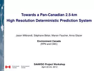
Towards a Pan-Canadian 2.5-km High Resolution Deterministic Prediction System. Jason Milbrandt, Stéphane Bélair, Manon Faucher, Anna Glazer Environment Canada (RPN and CMC). SAAWSO Project Workshop April 22-24, 2012. Modeling Systems and Applications at CMC / RPN.

E N D
Towards a Pan-Canadian 2.5-km High Resolution Deterministic Prediction System Jason Milbrandt, Stéphane Bélair, Manon Faucher, Anna Glazer Environment Canada (RPN and CMC) SAAWSO Project Workshop April 22-24, 2012
Environment Canada's NWP Model GEM (Global Environmental Multiscale) Various grid configurations: Global Variable Global Uniform • non-hydrostatic • fully compressible • semi-implicit • semi-Lagrangian • one-way self-nesting • staggered vertical grid (Charney-Phillips) Yin-Yang Limited Area (LAM) Côté et al. (1998) Mon. Wea. Rev.
LAM ≠ High Resolution Model LAM = Limited Area Model t = final t = 0 … Initial Conditions / Boundary Conditions Boundary Conditions fields from driving model
Environment Canada’s HRDPS (High Resolution Deterministic Prediction System) • 4 “full-time” grids • 1 “seasonal” grid • z = 2.5 km • 58 levels (staggered) • one 24-h daily run (per domain) • downscaled from RDPS-10 forecast • Li-Barker radiation • Milbrandt-Yau 2-moment microphysics 2 x 42-h integrations
Environment Canada’s HRDPS (High Resolution Deterministic Prediction System) • 1997: Project initiated by CMC/RPN (HiMAP) • Since 1999: Collaboration with PNR • Summer 2001: ELBOW project (MRB and Ontario region) • Since 2002: Collaboration with PYR • Since 2004: Collaboration Quebec region • Other related experimental systems: • 2001: MAP • 2007: MAP-DPHASE • 2008-09: UNSTABLE • 2008-10: Lancaster Sound • 2010: Vancouver 2010 Winter Olympics/Paralympics • 2014: Sochi 2014 Winter Olympics/Paralympics • 2015: Pan-American Games
Experimental EAST, MARITIME, ARCTIC Runs • 1 LAM-2.5km runs per day, 24-h • Nested from 6-h forecasts of 00z-REG-10 06 18 06 18 00 12 18 00 12 00 RDPS-10 LAM-10 HRDPS LAM-2.5
Operational WEST Runs • 2 LAM-2.5km runs per day, 42-h • Nested from 6-h forecasts of 00z- and 12z-REG-10 runs 06 18 06 18 00 12 18 00 12 00 RDPS-10 LAM-10 HRDPS RUN 1 LAM-2.5 RDPS-10 LAM-10 HRDPS RUN 2 LAM-2.5
A L M W E LAM2.5 windows: West (W), East (E), Maritimes (M), Lancaster (L), Arctic (A) N1 (ni x nj = 2904 x 1674) N2 (ni x nj = 2524 x 1334)
HRDPS Configuration • Future: • single grid (2.5 km) • - 4 x 48-h • 70 - 80 levels • IC surface fields from CaLDAS • upgraded microphysics • upper-air assimilation cycle • Current: (near future) • multi-grid (2.5 km) • - 2 x 42-h (west domain) • - 1 x 24-h (other domains) • downscaled from RDPS • 58 levels • IC surface fields from ISBA Next generation HRDPS • LAM 250-m grids (e.g. over cities)
HRDPS Future Plans • Operational WEST-2.5 domain • operational status of WEST; 2 x 42-h • upgrade of GEM version • National-2.5 – STAGE 1 • single, national grid • 2 x 48-h • increased vertical resolution • high-resolution surface fields (CaLDAS) • upgrade to microphysics • reduced spin-up (recycling PHY bus) • 2014 • National-2.5 – STAGE 2 • 4 x 48-h • upper-air data assimilation cycle (En-Var*) • 2016 * Buehner et al. (2010a,b)
Advantages of a cloud-scale deterministic NWP system: • Topographic forcing is better resolved • orography, vegetation, land-water boundaries • 2. Better physics • high-res surface data assimilation • no need for a CPS • can use a detailed microphysics scheme • Improved ability to forecast high-impact weather
The CANADIAN LAND DATA ASSIMILATION SYSTEM (CaLDAS*) IN OUT Ancillary land surface data Land surface initial conditions for NWP and hydro systems ISBA LAND-SURFACE MODEL Orography, vegetation, soils, water fraction, ... xb ASSIMILATION Land surface conditions for atmospheric assimilation systems Atmospheric forcing y OBS (with ensemble Kalman filter approach) T, q, U, V, Pr, SW, LW Observations Current state of land surface conditions for other applications (agriculture, drought, ... xa = xb+ K { y – H(xb) } Screen-level (T, Td) Surface stations snow depth L-band passive (SMOS,SMAP) MW passive (AMSR-E) Multispectral (MODIS) Combined products (GlobSnow) with K = BHT ( HBHT+R)-1 *Carrera et al. (2012) (to be submitted to J. Hydromet)
MOIST PROCESSES • OUTPUT: • Latent heating • Hydrometeors • (cloud, rain, ice,…) • qc, qr, qi, ... INPUT: w, T, p, qv For NWP models at the “convective scale” (x < 4 km), no longer need a CPS – clouds are considered to be resolved cloud / precipitation processes are treated by a grid-scale condensation scheme Single cloudy grid element – interaction with NWP model: qc, qr, qi, ...
VAPOR NUvc, VDvc NUvi, VDvi VDvr VDvs CLci, MLic, FZci CLOUD ICE CLcs CNig CNis, CLis CNcr, CLcr self- collection self- collection VDvh VDvg MLsr, CLsr RAIN SNOW CLsr CLrs CLcg CLri CLir CLrh, MLhr,SHhr CLih MLgr CLsh CLch CNsg CLsr-h CLsr-g GRAUPEL HAIL CLir-g CLir-g CNgh SEDIMENTATION SEDIMENTATION 2-Moment Microphysics Scheme* • Six hydrometeor categories: • 2 liquid: cloud, rain • 4 frozen: ice, snow, graupel, hail For each category x = c, r, i, s, g, h: Prognostic variables qx, Nx (12) * Milbrandt and Yau (2005a,b)
Mean-Mass Diameters, Dmx CLOUD (CLW) RAIN 10 – 30 microns (maritime CCN) 0.1 – 1 mm STRATIFORM RAIN DRIZZLE ICE (pristine crystal) 0.1 – 4 mm SNOW (large crystals / aggregates) 10 – 50 microns RIME-SPLINTERING 0.5 – 2 mm HAIL (ice pellets) GRAUPEL < 0.5 mm
Precipitation types from microphysics : RN1 – Liquid Drizzle RN2 – Liquid Rain FR1 – Freezing Drizzle FR2 – Freezing Rain SN1 – Ice Crystals SN2 – Snow SN3 – Graupel (snow pellets) PE1 – Ice Pellets (re-frozen rain) PE2 – Hail (total) PE2L – Large Hail
3D fields for VISIBILITYdue to fog, rain, and snow (parameterizations based on observations taken during FRAM) km VIS1 (liquid fog) VIS1 = f (qc,Nc) km VIS2 (rain) VIS2 = f (RRN2) km VIS3 (snow) VIS3 = f (RSN2) *Gultepe and Milbrandt (2007)
3D fields for VISIBILITYdue to fog, rain, and snow (parameterizations based on observations taken during FRAM) km VIS1 (liquid fog) VISIBILITY due to the combined effects of liquid FOG, RAIN, and SNOW: km VIS2 (rain) km VIS3 (snow)
3D fields for VISIBILITYdue to fog, rain, and snow (parameterizations based on observations taken during FRAM) km VIS1 (liquid fog) VIS (fog + rain + snow) km km VIS2 (rain) km km VIS3 (snow) 0.995
Real-Time Verification Examples (from SNOW-V10 site) Visibility (m)
Experimental EAST, MARITIME, ARCTIC Runs • 1 LAM-2.5km runs per day, 24-h • Nested from 6-h forecasts of 00z-REG-15 06 18 06 18 00 12 18 00 12 00 RDPS-15 LAM-15 HRDPS LAM-2.5
Recycling of Hydrometeor Fields 06 18 06 18 00 12 18 00 12 00 RDPS-10 ICs from RDPS analysis FLOW fields Consecutive 6-h runs (LAM-2.5) CLOUD fields ICs from 6-h forecast of previous 2.5-km run (cycle)
Recycling of Hydrometeor Fields 06 18 06 18 00 12 18 00 12 00 RDPS-10 ICs from RDPS analysis FLOW fields Consecutive 6-h runs (LAM-2.5) HRDPS CLOUD fields ICs from 6-h forecast of previous 2.5-km run (cycle)
CURRENT SET-UP of Deterministic NWP System 10 km m 2.5 km 1 km 250 m Configuration for FROST-2014
DEMOS – 24 Jan 2013 (heavy rain/snow) Near-surface winds: 2.5 km
DEMOS – 24 Jan 2013 (heavy rain/snow) Near-surface winds: 1 km
DEMOS – 24 Jan 2013 (heavy rain/snow) Near-surface winds: 250 m
DEMOS – 24 Jan 2013 (heavy rain/snow) 24-h Accumulated SNOW mm 2.5 km 1 km 250 m
DEMOS – 24 Jan 2013 (heavy rain/snow) 24-h SNOW 24-h RAIN Differences are not due to precipitation phase; 2.5-km run appears to underestimate the orographic enhancement 2.5 km 1 km 250 m