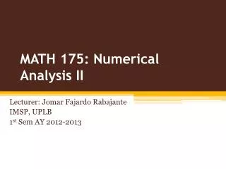
MATH 175: NUMERICAL ANALYSIS II
MATH 175: NUMERICAL ANALYSIS II. Lecturer: Jomar Fajardo Rabajante 2 nd Sem AY 2012-2013 IMSP, UPLB. STIFF ODEs.

MATH 175: NUMERICAL ANALYSIS II
E N D
Presentation Transcript
MATH 175: NUMERICAL ANALYSIS II Lecturer: Jomar Fajardo Rabajante 2ndSem AY 2012-2013 IMSP, UPLB
STIFF ODEs Remember that in our discussion from Variable Step-Size Methods, I told you that if h* becomes very small (say 10^-10) then halt the process. This is an indicator that your IVP might be stiff! There is no precise definition of stiffness but one instance that stiffness may occur is when solution to your IVP changes values drastically (slopes are too steep).
STIFF ODEs There are methods that for some h>stab, the method is unstable (where stab is the value of h at the boundary between stability and instability). Example: Given the following system of ODE, we need to choose h<0.2 in Euler’s method, so that we can get stable solutions. (Note: h<0.2 only gives us stability and not yet our desired accuracy.)
STIFF ODEs But sometimes we do not want our step size to be so small and sacrifice our computing time just to attain stability (especially when our time period considered is to wide). We want method that has larger stability region (graphed in a complex plane).
Stability Region for Backward Euler The shaded area is the stability region.
STIFF ODEs Note: Stiffness is a property of the ODE not of the numerical methods we have discussed (remember that all our discussed methods are consistent and convergent as h0). It is just for stiff ODEs, we cannot endure having very small h because of computational concerns. However, note that for Implicit Trapezoidal and Backward Euler’s methods, the left-hand side of their complex planes are shaded. These mean that they are A-stable methods, i.e. for any value of hthe approximates will converge to the long-term behavior of the solution.
Euler’s method requires tiny step Note: this is not the solution to our previous example.
Euler’s method with too large a step Note: this is not the solution to our previous example.
Large steps OK with Backward Euler’s Note: this is not the solution to our previous example.
Very large steps OK, too for Backward Euler’s Note: this is not the solution to our previous example.
Numerical Methods (Implicit) for Stiff ODEs One way to solve stiff ODEs is to bring information from the right side of the interval [ti, ti+h] instead of relying solely on the left side. • We have already seen the Implicit Trapezoidal method. Now, we will see Backward Euler’s Method (Implicit Euler’s Method). • Implicit R-K methods are known to be A-stable. • Berkeley Madonna uses Rosenbrock Method. Note: Implicit methods can be made adaptive.
BACKWARD EULER’S METHOD Example 1: Given the following IVP:
BACKWARD EULER’S METHOD Notice that we need to do some root-finding to get the approximates. Example 2: Then solve for wi+1 using Chapter 1, use wi as initial guess.
BDF Actually, Backward Euler’s Method is a 1st order Backward Differentiation Formula (BDF). The 2nd order BDF is