Numerical Analysis for Engineers
Numerical Analysis for Engineers . Eng. Muhannad Al- Jabi. Analytical and Numerical Solutions :. Numerical methods are techniques by which mathematical problems are formulated so that they can be solved with arithmetic operations. Approximations and Round-Off Errors.

Numerical Analysis for Engineers
E N D
Presentation Transcript
Numerical Analysis for Engineers Eng. Muhannad Al-Jabi
Analytical and Numerical Solutions: • Numerical methods are techniques by which mathematical problems are formulated so that they can be solved with arithmetic operations. Eng. Muhannad Al-Jabi
Approximations and Round-Off Errors • For many engineering problems, we cannot obtain analytical solutions. • Numerical methods yield approximate results, results that are close to the exact analytical solution. We cannot exactly compute the errors associated with numerical methods. • Only rarely given data are exact, since they originate from measurements. Therefore there is probably error in the input information. • Algorithm itself usually introduces errors as well, e.g., unavoidable round-offs, etc … • The output information will then contain error from both of these sources. • How confident we are in our approximate result? • The question is “how much error is present in our calculation and is it tolerable?” Eng. Muhannad Al-Jabi
Accuracy. How close is a computed or measured value to the true value • Precision (or reproducibility). How close is a computed or measured value to previously computed or measured values. • Inaccuracy(or bias). A systematic deviation from the actual value. • Imprecision(or uncertainty). Magnitude of scatter. Eng. Muhannad Al-Jabi
Significant Figures • Number of significant figures indicates precision. Significant digits of a number are those that can be used with confidence, e.g.,the number of certain digits plus one estimated digit. 53,800 How many significant figures? 5.38 x 1043 5.380 x 1044 5.3800 x 1045 Zeros are sometimes used to locate the decimal point not significant figures. 0.00001753 4 0.0001753 4 0.001753 4 Eng. Muhannad Al-Jabi
I can say the speed is between 48.5 and 48.9 km/h. Thus, we have a 3-significant figure reading. One might say the speed is between 48 and 49 km/h. Thus, we have a 2-significant figure reading. Eng. Muhannad Al-Jabi
Rules regarding the zero: • Zeros within a number are always significant: 5001 and 50.01 have 4 significant figures • Zeros to the left of the first nonzero digit in a number are not significant: 0.00001845, 0.0001845, 0.001845 have 4 significant figures • Trailing zeros are significant: 6.00 has 3 sig. figures. • 45300 may have 3, 4, or 5 sig. figures, we can know if the number is written in the scientific notation: 4.53×10⁴ has 3 sig. figures 4.530×10⁴ has 4 sig. figures 4.5300×10⁴ has 5 sig. figures Eng. Muhannad Al-Jabi
Error Definitions True Value = Approximation + Error Et = True value – Approximation (+/-) True error Eng. Muhannad Al-Jabi
For numerical methods, the true value will be known only when we deal with functions that can be solved analytically (simple systems). In real world applications, we usually not know the answer a priori. Then • Iterative approach, example Newton’s method Eng. Muhannad Al-Jabi
Use absolute value. • Computations are repeated until stopping criterion is satisfied. • If the following criterion is met you can be sure that the result is correct to at least n significant figures. Pre-specified % tolerance based on the knowledge of your solution Eng. Muhannad Al-Jabi
Round-off Errors • Numbers such as p, e, or cannot be expressed by a fixed number of significant figures. • Computers use a base-2 representation, they cannot precisely represent certain exact base-10 numbers. • Fractional quantities are typically represented in computer using “floating point” form, e.g., Integer part exponent mantissa Base of the number system used Eng. Muhannad Al-Jabi
Word • How are numbers represented in computers? • Numbers are stored in what is called ‘word’. A word has a number of bits, each bit holds either 0 or 1. • For example, -173 is presented on a 16-bit computer as Eng. Muhannad Al-Jabi
On a 16-bit computer, the range of numbers that can be represented is between -32,768 and 32,767. Eng. Muhannad Al-Jabi
156.78 (normal form) 0.15678×10³(floating point form) Word Floating Point Representation Eng. Muhannad Al-Jabi
156.78 0.15678x10³ in a floating point base-10 system Suppose only 4 decimal places to be stored • Normalized to remove the leading zeroes. Multiply the mantissa by 10 and lower the exponent by 1 0.2941 x 10⁻¹ Additional significant figure is retained Eng. Muhannad Al-Jabi
Therefore for a base-10 system 0.1 ≤m<1 for a base-2 system 0.5 ≤m<1 • Floating point representation allows both fractions and very large numbers to be expressed on the computer. However, • Floating point numbers take up more room. • Take longer to process than integer numbers. • Round-off errors are introduced because mantissa holds only a finite number of significant figures. Eng. Muhannad Al-Jabi
Rounding • Rounding up is to increase by one the digit before the part that will be discarded if the first digit of the discarded part is greater than 5. • If it is less than 5, the digit is rounded down. • If it is exactly 5, the digit is rounded up or down to reach the nearest even digit. • Round 1.14 to one decimal place: 1.1 • Round 1.15 to one decimal place: 2.2 • Round 21.857 to one decimal place: 21.8 Eng. Muhannad Al-Jabi
Chopping Example: p=3.14159265358 to be stored on a base-10 system carrying 7 significant digits. p=3.141592 chopping error et=0.00000065 If rounded p=3.141593 et=0.00000035 • Some machines use chopping, becauserounding adds to the computational overhead. Since number of significant figures is large enough, resulting chopping error is negligible. Eng. Muhannad Al-Jabi
Truncation Errors and the Taylor Series Eng. Muhannad Al-Jabi
Taylor’s Theorem If the function f and its first n+1 derivatives are continuous on an interval containing a and x, then the value of the function at x is given by: where the remainder Rn is defined as Eng. Muhannad Al-Jabi
Using Taylor’s Theorem, we can approximate any smooth function by a polynomial. • The zero-order approximation of the value of f(xi+1) is given f(xi+1)f(xi) • The first-order approximation is given by f(xi+1)f(xi) + f '(xi)(xi+1-xi) Eng. Muhannad Al-Jabi
The complete Taylor series is given by The remainder term is where is between xiand xi+1 Eng. Muhannad Al-Jabi
Notes • We usually replace the difference (xi+1 - xi) by h. • A special case of Taylor series when xi = 0 is called Maclaurin series. Eng. Muhannad Al-Jabi
Solution h = /3 - /4 = /12 Zero-order approximation: f(/3) cos (/4) = 0.707106781 t = First-order approximation: f(/3) cos (/4) – (/12) sin (/4) = 0.521986659 t = -4.4% See Table 4.1 Example Use Taylor series expansions with n = 0 to 6 to approximate f(x) = cos x near xi = /4 at xi+1 = /3. Eng. Muhannad Al-Jabi
To get more accurate estimation of f(xi+1), we can do one or both of the following: • add more terms to the Taylor polynomial • reduce the value of h. Eng. Muhannad Al-Jabi
Roots of equations All Iterative Eng. Muhannad Al-Jabi
Bracketing Methods(Or, two point methods for finding roots)Chapter 5 • Two initial guesses for the root are required. These guesses must “bracket” or be on either side of the root. == > Fig. 5.1 • If one root of a real and continuous function, f(x)=0, is bounded by values x=xl, x=xu then f(xl) . f(xu) <0. (The function changes sign on opposite sides of the root) Eng. Muhannad Al-Jabi
No answer (No root) Two roots( Might work for a while!!) Nice case (one root) Discontinuous function. Need special method Oops!! (two roots!!) Three roots ( Might work for a while!!) Figure 5.2 Figure 5.3 Eng. Muhannad Al-Jabi
The Bisection Method For the arbitrary equation of one variable, f(x)=0 • Pick xl and xu such that they bound the root of interest, check if f(xl).f(xu) <0. • Estimate the root by evaluating (xl+xu)/2. • Find the pair • If f(xl). f[(xl+xu)/2]<0, root lies in the lower interval, then xu=(xl+xu)/2 and go to step 2. Eng. Muhannad Al-Jabi
If f(xl). f[(xl+xu)/2]>0, root lies in the upper interval, then xl= [(xl+xu)/2, go to step 2. • If f(xl). f[(xl+xu)/2]=0, then root is (xl+xu)/2 and terminate. • Compare es with ea • If ea<es, stop. Otherwise repeat the process. Eng. Muhannad Al-Jabi
Figure 5.6 Eng. Muhannad Al-Jabi
Evaluation of Method Advantages • Easy • Always find root • Number of iterations required to attain an absolute error can be computed a priori. Disadvantages • Slow • Know a and b that bound root • Multiple roots • No account is taken of f(xl) and f(xu), if f(xl) is closer to zero, it is likely that root is closer to xl . Eng. Muhannad Al-Jabi
How Many Iterations will It Take? • Length of the first Interval Lo=b-a • After 1 iteration L1=Lo/2 • After 2 iterations L2=Lo/4 • After k iterations Lk=Lo/2k Eng. Muhannad Al-Jabi
If the absolute magnitude of the error is and Lo=2, how many iterations will you have to do to get the required accuracy in the solution? Eng. Muhannad Al-Jabi
The False-Position Method(Regula-Falsi) • If a real root is bounded by xl and xu of f(x)=0, then we can approximate the solution by doing a linear interpolation between the points [xl, f(xl)] and [xu, f(xu)] to find the xr value such that l(xr)=0, l(x) is the linear approximation of f(x). == > Fig. 5.12 Eng. Muhannad Al-Jabi
Procedure • Find a pair of values of x, xl and xu such that fl=f(xl) <0 and fu=f(xu) >0. • Estimate the value of the root from the following formula (Refer to Box 5.1) and evaluate f(xr). Eng. Muhannad Al-Jabi
Use the new point to replace one of the original points, keeping the two points on opposite sides of the x axis. If f(xr)*f(xu)<0 then xl=xr If f(xr)*f(xl)<0 then xu=xr If f(xr)=0 then you have found the root and need go no further! Eng. Muhannad Al-Jabi
See if the new xl and xu are close enough for convergence to be declared. If they are not go back to step 2. • Why this method? • Faster • Always converges for a single root. See Sec.5.3.1, Pitfalls of the False-Position Method Note: Always check by substituting estimated root in the original equation to determine whether f(xr) ≈ 0. Eng. Muhannad Al-Jabi
example Determine the real roots of A)By using the bisection method B)By using the false position method Eng. Muhannad Al-Jabi
Solution of part A Eng. Muhannad Al-Jabi
Solution of part B Eng. Muhannad Al-Jabi
Open Methods • Open methods start with a starting point or the initial guess. • Because the open methods do not bracketing the root, they may be converges or diverges. • On the other hand open methods are faster in finding the root. ( more efficient). • Open methods are:- simple fixed point iteration, Newton Raphson, Secant and multiple roots Eng. Muhannad Al-Jabi
Simple fixed point iteration • Rearrange the function so that x is on the left side of the equation: • Fixed-point methods may sometime “diverge”, depending on the stating point (initial guess) and how the function behaves. Eng. Muhannad Al-Jabi
Example: Eng. Muhannad Al-Jabi
Convergence • x=g(x) can be expressed as a pair of equations: y1=x y2=g(x) (component equations) • Plot them separately. Eng. Muhannad Al-Jabi
Fixed-Point Iteration Convergent Divergent Eng. Muhannad Al-Jabi
Conclusion • Fixed-point iteration converges if • When the method converges, the error is roughly proportional to or less than the error of the previous step, therefore it is called “linearly convergent.” Eng. Muhannad Al-Jabi