Decays - + + - n etc .
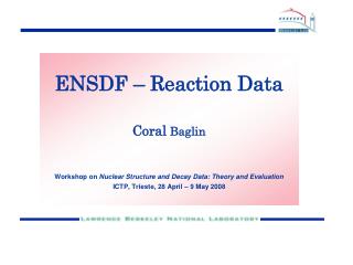
ENSDF Database Structure. ENSDF. …. A=1. A=294. A. …. Abs. Z min. Z. Z max. Ref. Adopted (best values) Q values Levels: (E, J , T1/2, , Q, config, excitn.) Gammas: (E, Br, Mult, ). Reactions (HI,xn ) (p,p’ ) (n, ) Coul. Exc. (,’) (d,p) etc. Decays - + +

Decays - + + - n etc .
E N D
Presentation Transcript
ENSDF Database Structure ENSDF .... …. A=1 A=294 A .... …. Abs Zmin Z Zmax Ref Adopted (best values) Q values Levels: (E, J, T1/2, , Q, config, excitn.) Gammas: (E, Br, Mult, ) Reactions (HI,xn) (p,p’ ) (n, ) Coul. Exc. (,’) (d,p) etc. Decays - ++ -n etc. 0 to ~6 datasets 1 dataset 0 to ~40 datasets
Summary • Principal Categories of Reactions. • Reactions in which gammas are not detected: • Stripping and Pickup Reactions • Multi-particle Transfer Reactions • Charge-Exchange Reactions • Inelastic Scattering • Coulomb Excitation (particles detected) • Resonance Reactions … • Reactions in which gammas are detected: • Summary of information available from -ray measurements • Inelastic Scattering • Nuclear Resonance Fluorescence • (light ion,xnyp) • (heavy ion,xnyp) • Particle Capture • Coulomb Excitation (’s detected)
Gammas not detected • Measured Quantities of Interest: • E(level) from particle energy spectrum or excitation function. • L – angular momentum transfer • S, C2S - spectroscopic factors • 2, 4 - deformation parameters (if model independent) • , i – total or partial widths for level • B(E), B(M ) – transition probabilities • J, T – spin, parity, isospin
Stripping and Pickup • Examples: • Stripping: (d,p), (,3He), (pol d,p), (3He,d), etc. • Pickup: (p,d), (3He,), (t,), etc. • Quantities to Record: • E(level), deduced by authors from charged particle spectrum. • L and S or C2S from authors’ DWBA analysis: • (d/d())exp= (d/d())DWBA x N x C2S’ • where S’=S (pickup) or • S’=S x (2Jf+1)/(2Ji+1) (stripping) • (d/d for one angle should be given in suitably relabeled S field when spectroscopic-factor information is not provided by authors.) • J from L±1/2 for polarised beam if vector analysing power shows clear preference between L+1/2 and L-1/2. • Relevant Documentation: • Target J (unless 0+) • Spectrum resolution (FWHM, keV) • Normalisation factor for DWBA analysis • Range of angles measured, lab or c.m. (but specify which).
Stripping and Pickup, ctd. • Deformed Nuclides; and lighter beams: • (d/d())exp / [(d/d())DWBA x 2N] = c2(jl)V2, • where c is amplitude of Nilsson state wavefunction for transferred nucleon, V is fullness factor describing partial filling of target nucleus orbitals. • The pattern of cross sections among rotational-band members may provide a characteristic fingerprint for a specific Nilsson configuration, enabling a set of levels to be assigned as specific J members of a band with that configuration if: • (i) the experimental fingerprint agrees well with that predicted by Nilsson-model wave functions, and • (ii) the fingerprint differs distinctly from those for other plausible configurations. • Example: (d/d(60)) calculated (1997Bu03) for 226Ra(t, )225Fr: • Orbital: 1/2[400] 1/2[530] 1/2[541] 3/2[402] 3/2[651] 3/2[532] Expt. Mixed • J=3/2 23 14 1.5 103 0.0 0.7 ~1.5 0.9 • J=5/2 7.6 0.2 13 4.6 0.03 6.2 14 10 • J=7/2 0.4 39 2.0 1.2 0.0 3.3 20 4.1 • J=9/2 0.05 0.4 33 0.05 2.0 26 ~45 49 • Reality (not so simple!): 3/2[532] Coriolis mixed with 1/2[541] fits , energy.
Multi-particle Transfer • Examples: • (p,t), (,d), (t,p), (,p), (6Li,d) …. • Quantities to Record: • E(level) • L – if angular distribution can be fitted by a unique value • Deduced Quantities: • J- from J(target)+L (vector sum) and if=(-1)Jf, for strong groups only in two-neutron, two-proton or –particle transfer. • (i.e., pairs of identical particles can be assumed to be transferred in relative s state for strong groups).
Charge-Exchange Reactions • Examples: • (p,n), (3He,t) • Quantities of interest: • E(level) • Isobaric analog state information. IAS
Inelastic Scattering • Examples: • (e,e’), (p,p’), (d,d’), (,’) (at projectile energies above the Coulomb barrier). • Quantities to Record: • E(level) • L – if angular distribution is fitted by unique L value • 2, 4 … - deformation parameters (if model independent); specify whether ‘charge’ or ‘nuclear’, if relevant (typically from (,’) or (e,e’)). • B(E), B(M ) – transition probabilities (typically from (e,e’)).
Coulomb Excitation (particles detected) • Examples: • (p,p’), (d,d’), (,’) with projectile energy below Coulomb barrier. • Quantities to Record: • E(level) • J: • determined if the excitation probability agrees with that calculated by Alder (1960Al23). • low energy Coulomb excitation is predominantly E2 • B(E) – for excitation (i.e., B(E)↑)
Resonance Reactions • Examples: • (p,p), (p,X), (,n) … (excitation function data, (E), d/d(,E)) • Quantities of interest: • E(level) – calculate from SP+E(p)(c.m.) or give as ‘SP+976.3’, etc., where 976.3 is E(p)(lab) for resonance; don’t use both notations within the same dataset. • Ep at resonance - can be given in relabeled ‘S’ or ‘L’ field. • Partial widths – can be given in comments or relabeled ‘S’ field. • Is this an isobaric analog state? (If so, specify state of which it is the analog). • Is this a giant resonance? (If so, which one?) • Any J information that can be deduced. • Note: • ENSDF is primarily concerned with bound levels, but includes all isobaric analog states, giant resonances, and unbound levels which overlap or give information on bound levels.
Reactions with Gammas Detected • Measured Quantities of Interest: • E - photon energy • I - relative intensity (or photon branching) • , K, … - electron conversion coefficients, usually from I(ce)/I; sometimes from intensity balance (note: this gives exp). • K/L, L1/ L3 … - ce subshell ratios • A2, A4 … - Legendre polynomial coefficients characterizing angular distribution (()) or angular correlation (()). • DCO ratio – directional correlation of gammas from oriented nuclei. • Asymmetry ratio - e.g., I(1)/I(2) • Linear polarization • Level T1/2 – from (t), DSAM, RDM, centroid-shift, delayed coincidence, etc., if measured in that reaction (state method used). • g-factor – include if measured in that reaction
Reactions with Gammas Detected – ctd. • Deduced Quantities of Interest: • E(level) – from least-squares adjustment of E (GTOL), avoiding E for lines that have uncertain or multiple placements whenever possible. Note serious misfits. • Band structure – indicate via band flags for levels. (Note: life will be easier if a given band has the same band-flag character in each dataset in the nuclide!). • Band configurations – justify when possible; band parameters may be informative, especially for K=1/2 bands. • J - it may be desirable to indicate authors’ values in the reaction dataset and add parentheses in Adopted Levels if insufficient (or no!) supporting arguments are available (but note major discrepancies). • Transition quadrupole moment (if authors give it; include on level comment record or in band description). • M - transition multipolarity • – mixing ratio (((L+1)-pole/(L-pole)), Krane-Steffen sign convention.
Gamma-ray Energies • Give measured energy and uncertainty (i.e., do not correct for recoil energy loss). • State source of data (unless obvious, e.g., if only one keynumber) • Uncertainties: if authors give uncertainty as: • (i) “0.3 keV for strong lines, 1 keV for weak or poorly resolved lines”; assign 0.3 to those which could be reasonably considered ‘strong’ and 1 to all others, but give authors’ statement in general comment on E and define the I that you consider ‘strong’ (or assign 1 keV to all). • (ii) “do not exceed 0.5 keV”; 0.5 could be assigned for all lines. • (iii) If no uncertainty is stated, point that out in a general comment [for the purpose of deducing E(level) using GTOL, a default of 1 keV (adjustable by user via control record at head of dataset) will be used and this should be noted in a comment on level energy] • If measured E not available but G record is needed in order to give other information, deduce it from level energy difference and remove recoil energy loss; give no ΔE and say where E came from.
Gamma-ray Intensities • Give relative intensities, if available (don’t renormalise so strongest is 100). • Don’t mix data from different reactions, or data from same reaction at different energies, when entering RI on G records (use different datasets instead, or include in comments or tabulation). • If branching ratios are measured independently (e.g., from coincidences), quote these also (e.g., in a comment); one set of data may be more precise than the other. • Give uncertainties whenever authors state them; if authors give both statistical and systematic uncertainties, show statistical on G record but state systematic in comment (so uncertainty in I ratios is not distorted). • If both prompt and delayed I are given, use separate datasets for them or give one set under comments. • For multiply-placed lines, specify whether quoted I has been suitably divided between placements (& (undivided) or @ (divided) in column 77).
Conversion Coefficients • Give measured K, L, etc., and subshell ratios (in comments or on continuation of G record); state how photon and ce intensity scales were normalised. • Quote experimental coefficients (usually ) obtained using intensity balance arguments (these are frequently buried in the text of a paper); specify as “from intensity balance at xxxx level”, where relevant. • Include (theory) on G record (from BrIcc) when needed for calculation or argument (or (theory)+(pair) if E > 1022 keV). Linear Polarisation linear polarisation data may be available from Compton polarimeter measurements of relative I in planes perpendicular and parallel to reaction plane. Such data may distinguish between electric and magnetic radiations.
Angular Distributions • I as a function of angle with respect to beam direction: • W()=1+A2P2(cos )+A4P4(cos )+ … • Include A2, A4 … ; these data are very important to evaluators and readers alike, as they provide information vital to transition multipolarity assignments. • Remember that these are signed quantities. • A2, A4 … depend on ΔJ, mixing ratio and degree of alignment /J, where is half-width of Gaussian describing the magnetic substate population. • /J is usually determined from measurements of W() for known ΔJ=2 transitions. However, many authors assume /J=0.3, for practical purposes. • /J affects only the magnitudes of A2, A4. • For high-spin states, W() is largely independent of J. • Alignment is reduced if level lifetime is not small. • W() can determine ΔJ but notΔ.
Angular Distributions – ctd. Typical values of A2, A4 for relative to beam direction if /J=0.3 (from B. Singh, McMaster University)
DCO Ratios • Directional Correlations of -rays from Oriented states of Nuclei • If K (known multipolarity) and U (unknown multipolarity) are measured in coincidence using detectors at angles 1 and 2 to the beam: • DCO=I(U(at 1) gated by K(at 2))/I(U(at 2) gated by K(at 1)) . • Sensitive to ΔJ, multipolarity and mixing ratio; independent of Δ. • Gating transitions are frequently stretched Q, but stretched D may also be used, so specify which was used. • Authors frequently indicate expected DCO values for stretched Q and stretched D transitions for the geometry used. It is helpful to state these. • Remember that identical values are expected for stretched Q and for D, ΔJ=0 transitions (although the latter are less common).
DCO Ratios – ctd. Typical DCO values for 1=37°, 2=79°, /J=0.3 (B. Singh, McMaster U.)
Multipolarity • L andΔ may be determined from measured subshell ratios or conversion coefficients. • L alone can be determined by angular distributions or DCO ratios or asymmetry ratios. • Δ may be determined by linear polarisation measurements. • When transition strengths are calculable (T1/2 and branching known),Recommended Upper Limits (RUL) can be used to rule out some multipolarities (e.g., a stretched Q transition for which B(M2)W exceeds 1 can be assigned as E2). Similarly, for a D+Q transition with large mixing, RUL may enable the rejection of E1+M2. • Assign Mult when measured information indicates a clear preference for that assignment; otherwise, let () or DCO data speak for themselves. (Exception: if no measurement exists but mult. is needed for some reason, use the [M1+E2], etc., type of entry.) • Mult determined for a doublet will be not reliable; it can be given in comment (with disclaimer), but not on G record.
Mixing Ratios • Include on G record whenever available. • Calculate from conversion electron data or () using the program DELTA, or from subshell ratios. • Rely on authors’ deductions from () , DCO or nuclear orientation data. • Note: In (HI,xn) studies, model-dependent values of are sometimes deduced from in-band cascade to crossover transition intensity ratios; these could be given in comments (stating relevant K) if considered really important, but should not be entered on G record. • Check that correct sign convention was used by authors. Convert to Krane-Steffen if not, and take special care if uncertainties are asymmetric (-2.3 +4-2 becomes +2.3 +2-4 upon sign reversal).
Inelastic Scattering (p,p’), (n,n’), etc.; beam energies > Coulomb barrier. Separate these datasets from those for (p,p’), (n,n’) … and from that for Coulomb excitation. Information of interest: typically E, I, (); maybe linear polarisation. Nuclear Resonance Fluorescence (,) and (,’) measurements with Bremsstrahlung spectrum; low momentum transfer so excite low-spin states (mainly E1 and M1, but some E2 excitation). • spectrum measured; areas of peaks at Ex0 and Ex1, combined with knowledge of N(Ex0), yields scattering cross sections from which width and branching information may be obtained. • asymmetry differentiates D and Q excitation • linear polarization differentiates M and E Ex1 (,’) Ex0 (,) Counts E Beam flux Endpoint E0 E
Nuclear Resonance Fluorescence – ctd. • (Integrated) scattering cross section Is (eV b) is often given: • Is = ((2J+1)/(2J0+1)) (0f /) (ħc/E)2 W()/4 • where J is g.s. spin, J0 is spin of excited level, is its total width and 0, f its decay widths for decay to the g.s. and the final state f (for elastic scattering, 0=f); W() represents the normalised angular distribution. Data are often taken at 127° where W=1 for D transitions. • Give 02/ values (extract if necessary) on L record (col. 65 (value), 75 (uncertainty)); relabel field. • If f /0 is measured, include relative branching on G records. • is calculable from: • (02/) / (0/ )2 • using known branching, or under the assumption =0+f (which needs to be stated). • Then: T1/2 (ps)= 0.456 / (meV); include on L record. • Propagate uncertainties with care!
(Light Ion,xnyp) • (p,xn), (3He, xn), (,p), etc. • Separate from (HI,xn) studies, whenever practical. • Separate from datasets in which gammas are not measured (e.g., do not combine (d,p) and (d,p)). (Heavy Ion,xnyp) • Relative intensities will be different for different reactions and also for a given reaction measured at different beam energies; in general, it will be simplest to use separate datasets for each study that provides significant I or branching data. • (HI,xn) reactions tend to populate yrast (lowest energy for given J) levels or near-yrast levels; populated states tend to have spins that increase as the excitation energy increases. • Use band flags to delineate deduced band structure. If authors give configuration for band, include this in band description.
(Heavy Ion,xnyp) – ctd. • Note inconsistencies in order, postulated J, configuration, etc., compared with other studies and especially with that in Adopted Levels, Gammas. • Beware of multipolarity and J assignments for which no supporting measurements exist. Sometimes, unmeasured values inserted in order to generate a RADWARE band drawing live on in the published table of data; these do not qualify as ‘measured data’! • Multipolarities determined as D, Q, D+Q, etc, by () or DCO are best left this way in the reaction dataset unless definite arguments exist (e.g., from RUL) to establish Δ; otherwise ‘D’ (strong J argument) and ‘(D)’ (weak J argument) become indistinguishable when written as, say, (M1). • Watch for and report statements of coincidence resolving time (or equivalent) since this might place a limit on level lifetime, thereby enabling RUL to be used to reject Δ=yes for a transition multipolarity. • For K=1/2 rotational bands, the decoupling parameter may give a clear indication of the Nilsson orbital involved in the band configuration.
(Heavy Ion,xnyp) – ctd. • For a deformed nucleus: if a cascade including J=2 and/or J=1 transitions is observed at high spin with regular energy progression, they can be assigned to a band with definite J assignments if at least one level J and one in-band transition with multipolarity E2 or M1(+E2) can be assigned independently. • For near-spherical nuclei: if a cascade of ΔJ=1 transitions is observed at high spin with regular energy progression, those transitions may be assigned as (M1) transitions within a common band. Exception: in rare cases, nuclei can have alternating parity bands (reflection asymmetry); for these, ΔJ=1, Δ=yes cascades occur. • Note, however, that octupole-deformed nuclei may exhibit an apparent band structure which is really two ΔJ=2 rotational sequences of opposite parity, connected by cascading E1 transitions. • Special Case: • Superdeformed band data are updated continuously in ENSDF by Balraj Singh (McMaster University). One should check ENSDF as one finishes one’s mass chain evaluation to be sure no SD-band data were added since the chain was downloaded for revision.
Capture Reactions • (p,), (n,) E=thermal, (n,) E=res, etc. • Use separate datasets for thermal and resonance n-capture data. • Primary and secondary transitions usually appear in the same dataset even if their intensities require different normalisations. • The J of the thermal neutron capture state(s) is J(target)±1/2(i.e., s-wave capture is assumed). • In thermal neutron capture, the multipolarity of a primary is E1, M1, M1+E2 or E2. • For resonance n capture, ENSDF does not include the resonances and their properties; it is adequate to just list the bound states fed, their interconnecting gammas and any conclusions concerning level J. • In average resonance n capture, inclusion of primary gammas and their reduced intensities (which carry information on final state J) is optional; a list of final level E and deduced J would suffice.
Coulomb Excitation • If authors determine matrix element values, give them in comments and calculate B(E) using • B(E) = |<M(E)>|2/ (2J0+1) where J0 is g.s. spin. • If authors give B(E)↓, convert it to B(E)↑ and include it with level information. (B(E; i→f)) = B(E: f→i) x (2Jf+1)/(2Ji+1)) • In the strongly-deformed region, a cascade of E2 transitions with enhanced transition probabilities (B(E2)W > 10) provides definitive evidence for a rotational band and for the sequence of J values, provided the J of one level is known independently. • Calculate level T1/2 from B(E) and adopted -ray properties when possible. • Occasionally, mixing ratio or nuclear moment information can be extracted from matrix elements. • Clearly indicate the direction for any B(E) values given.