Download
1 / 29
300 likes | 704 Views
Proximity Greedy triangulation, star of spokes. “Star of spokes” greedy triangulation The simple greedy triangulation had two phases: 1. Generation and presort of possible edges. O ( N 2 log N ) time. 2. Determining if each possible edge belongs in the triangulation. O ( N 3 ) time.

E N D
ProximityGreedy triangulation, star of spokes “Star of spokes” greedy triangulation The simple greedy triangulation had two phases: 1. Generation and presort of possible edges. O(N2 log N) time. 2. Determining if each possible edge belongs in the triangulation. O(N3) time. The “star of spokes” algorithm reduces the second phase to O(N2 log N) overall by “processing” each of the O(N2) possible edges in O(log N) time. Here “processing” means to test a possible edge for intersection with edges already in the triangulation. We will see a way to perform that test in O(log N) time. That time suggests a search data structure of some kind.
ProximityGreedy triangulation, star of spokes Star of spokes Suppose the current possible edge is edge p1pi. Consider a set of edges connecting p1 to every other point in S. These edges, called spokes, are not in the triangulation, there are defined for the search structure. The point p1 and the spokes are together referred to as STAR(p1), the “star of spokes” of p1. The spokes are ordered, say counterclockwise, and they subdivide the 2 angle around p1 into N - 1 angular intervals, called sectors. pi p1
ProximityGreedy triangulation, star of spokes Triangulation edges and sectors Suppose edge pjpk is already part of the triangulation, i.e., a triangulation edge. It spans a set of consecutive sectors relative to p1, and the same is true for any plS - {pj, pk}. Observe that because triangulation edges run from point to point, and points define sectors, edges always entirely span sectors, rather than partially spanning them. Note also that triangulation edges do not intersect each other (by definition), so the triangulation edges present in each sector of STAR(pl) plS can be ordered from pl outwards. pi pj p1 pk
ProximityGreedy triangulation, star of spokes What to check Recall that edge p1pi is the possible triangulation edge that is being tested for intersection with other triangulation edges. Assume that in STAR(p1) point pi is located in sector pkp1pj. To determine whether edge p1pi can be added to the triangulation, it must be determined if edge p1pi intersects any other triangulation edge. It is sufficient to check those triangulation edges that span sector pkp1pj, and if there are > 1 such edges, it is sufficient to check the one closest to p1 in that sector. Conceptually, if pi is closer to p1 than the closest spanning edge, edge p1pi can be added; if not, it cannot. For each sector of STAR(pl) for every plS, the closest triangulation edge must be maintained. Preparata calls this “a special case of planar point location”. pi pj p1 pk
ProximityGreedy triangulation, star of spokes Example situation The figure shows STAR(p1) in some typical situation. The heavy edges are triangulation edges, and the lighter edges are spokes. A possible triangulation edge p1pi can be added iff pi is in the shaded area.
ProximityGreedy triangulation, star of spokes Search data structure The data structure to store the spanning edge for each sector in STAR(pl) for plS must support two operations: 1. Query to determine if a possible triangulation edge intersects a spanning triangulation edge. 2. Insertion of new triangulation edges. The second operation indicates that a dynamic data structure is needed. We would like the operations to execute in O(log N) time. Because each insertion involves a sequence of consecutive spanned sectors a segment tree is suggested.
ProximityGreedy triangulation, star of spokes Sectors of STAR(pl) The sectors of STAR(pl) can be numbered in counterclockwise order, from 1 to N - 1. 3 1 2 2 4 1 3 4 pl sector 5 9 5 Point in CCW sequence 9 6 8 7 7 6 8
[1,10] [1,5) [5,10] [1,3) [3,5) [5,7) [7,10] [8,10] [4,5) [7,8) [1,2) [2,3) [3,4) [5,6) [6,7) 1 2 3 4 5 6 7 [8,9) [9,10] 8 9 ProximityGreedy triangulation, star of spokes Segment tree for STAR(pl) The sectors of STAR(pl) are represented as the N - 1 leaves of a segment tree, referred to as Tl, defined for interval [1,N]. Each node v of Tl has a field e(v) that stores an edge. Field e(v) identifies the triangulation edge closest to to pl in the sector(s) that correspond to the node v.
ProximityGreedy triangulation, star of spokes Insertion When an edge pipj (arbitrary, not pipj from earlier figure) is to be added to the triangulation, it is inserted into the segment tree Tl representing STAR(pl) for every plS, li, j. During a single insertion, at each allocation node v in the segment tree Tl, edge pipj is tested against the edge identified by e(v). If edge pipj is closer, e(v) is updated to identify edge pipj. No ambiguity about “closest” is possible, because 1. Triangulation edges do not intersect. 2. An edge is only allocated to a node v if it spans all the sectors for that node. 1 2 not possible Test and update of e(v) take constant time at each node. Insertion into the segment tree will visit O(log N) nodes, so the insertion time is O(log N).
ProximityGreedy triangulation, star of spokes Query To test if edge pipj (arbitrary, not pipj from earlier figure) intersects any edge of the triangulation, search segment tree Tl representing STAR(pl) with the number of the sector contain pj. The search will trace a single path of nodes in Ti from root to leaf. At each node v on the path, test edge pipj for intersection with e(v). If an intersection is found, stop. If the search reaches a leaf without finding any intersections, accept edge pipj for the triangulation (add it to every segment tree). A segment tree has depth O(log N), so there are O(log N) nodes visited during the query. The intersection test at each one require O(1) time. The query requires O(log N) time. pj pj pi
ProximityGreedy triangulation, star of spokes “Star of spokes” greedy triangulation analysis Time: O(N2 log N); O(N2 log N) for presort of all possible edges, O(N2) edges O(log N) processing for each Storage O(N2); O(N) storage for the segment tree for each of N points
ProximityConstrained triangulation Problem definition CONSTRAINED TRIANGULATION INSTANCE: Set S = {p1, p2, ..., pN} of N points in the plane, and set E = { {pi, pj}, … } of nonintersecting edges on S. QUESTION: Join the points in S with nonintersecting straight line segments so that every region internal to the convex hull of S is a triangle and every edge of E is in the triangulation. For this problem, optimization (e.g., edge length minimization) is not required. A greedy method will work (with the edges in E put into the triangulation initially), but performance is not optimum. Delaunay triangulation is not easily adapted.
ProximityConstrained triangulation Assumptions Given S and E, assume: 1. We will triangulate not S, but instead the interior of the smallest axis-parallel rectangle that encloses S, considering S and E. The enclosing rectangle is denoted rect(S). This adds 4 points beyond those of S to be triangulated. 2. No two points of S have the same ordinate (y coordinate) except the corners of rect(S). The procedure can be modified to eliminate this assumption, at the cost of introducing special cases. rect(S) edge in E point in S
ProximityConstrained triangulation S, E (1) Inscribe S in minimum enclosing axis parallel rectangle. O(N) PSLG rect(S), S, E (2) Regularize rect(S), S, E. O(N log N) Each region within regularized rect(S), S, E is a monotone polygon. Regularized rect(S), S, E (3) Decompose regularized rect(S), S, E into monotone polygons. O(N) Monotone polygon (4) Triangulate monotone polygons. O(N) Triangulation of rect(S) Comments Steps (1) and (3) are very simple. Step(2) was previously described. Step(4) will be explained.
ProximityConstrained triangulation Regularization of rect(S) The regularization process operates on rect(S), S, and E. These together form a PSLG. To regularize, apply the plane-sweep algorithm to regularize a PSLG described earlier for the chain method of point location. Regularization requires O(N log N) time. After regularization, these properties hold: (i) No two edges intersect, except at vertices. (ii) Each vertex (except those with largest y coordinate) is joined directly to at least one vertex with a larger y coordinate. (iii) Each vertex (except those with smallest y coordinate) is joined directly to at least one vertex with a smaller y coordinate. rect(S) edge in E point in S edgeadded during regularization
ProximityConstrained triangulation Monotone polygons A polygon P is monotone w. r. t. a straight line l if P is simple and its boundary is the union of two chains monotone w.r.t. l. The regularization process partitions the interior of rect(S) into a set of polygons, each of which is monotone. For a proof, see Preparata pp. 238-239. Furthermore, they are monotone w.r.t. the y axis, i.e., the line of monotonicity l is the y axis. The top and bottom edges of rect(S) are exceptions to the y axis monotonicity, and are handled as special cases. P1 P2 P3 P4
ProximityConstrained triangulation Triangulating a monotone polygon, introduction The algorithm to triangulate a monotone polygon depends on its monotonicity. Developed in 1978 by Garey, Johnson, Preparata, and Tarjan, it is described in both Preparata pp. 239-241 (1985) and Laszlo pp. 128-135 (1996). The former uses y-monotone polygons, the latter uses x-monotone. Initialization Sort the N vertices of monotone polygon P in order by decreasing y coordinate. (Here N is the number of vertices of P, not S.) The sort can be done in O(N) time, not O(N log N), by merging the two monotone chains of P. Let u1, u2, …, uN be the sorted sequence of vertices, so y(u1) > y(u2) > … > y(uN). Because of the regularization process and the monotonicity of P, for every ui 1 i < N there exists uj 1 < jN such that edge uiujis an edge of P.
ProximityConstrained triangulation Description of the processing The algorithm processes one vertex at a time in order of decreasing y coordinate, creating diagonals of polygon P. Each diagonal bounds a triangle, and leaves a polygon with one less side still to be triangulated. Stack The algorithm uses a stack to store vertices that have been visited but not yet connected with a diagonal. The stack content is v1, v2, …, vi, where v1 is the bottom and vi the top of the stack. At any time during the execution, there are two invariants: 1. The vertices v1, v2, …, vi on the stack from a chain on the boundary of P, where y(v1) > y(v2) > … > y(vi). 2. If i 3, angle vjvj+1vj+2 for 1 ji - 2.
ProximityConstrained triangulation Algorithm By “adjacent” we mean connected by an edge in P. Recall that v1 is the bottom of the stack, vi is the top. 1. Push u1 and u2 on the stack. 2. j = 3 /* j is index of current vertex */ 3. u = uj 4. Case (i): u is adjacent to v1 but not vi. add diagonals uv2, uv3, …, uvi. pop vi, vi-1, …, v1 from stack. push vi, u on stack. Case (ii): u is adjacent to vi but not v1. while i > 1 and angle uvivi-1 < add diagonal uvi-1 pop vi from stack endwhile push u Case (iii): u adjacent to both v1 and vi. add diagonals uv2, uv3, …, uvi-1. exit 5. j = j + 1 Go to step 3.
v1 v2 v3 v4 = vi top of stack u ProximityConstrained triangulation Algorithm cases Case (i): u is adjacent to v1 but not vi. v1 v2 v3 v4 = vi top of stack u Case (ii): u is adjacent to vi but not v1. v1 v2 v3 v4 v5 = vi top of stack u Case (iii): u adjacent to both v1 and vi.
v1 v1 v2 v2 v3 u u 2, Case (ii) 1, initial v1 v2 v3 v4 v1 u v2 u 3, Case (ii) 4, Case (i) ProximityConstrained triangulation Example, 1
v1 v1 v2 v2 u v3 u 5, Case (ii) 6, Case (ii) v1 v2 v3 v4 u 7, Case (ii) ProximityConstrained triangulation Example, 2 v1 v2 v3 8, Case (ii) u
ProximityConstrained triangulation Example, 3 9, Case (iii) 10, final
ProximityConstrained triangulation Proof of correctness The correctness of the algorithm depends on the fact that all the added diagonals lie inside the polygon P. For details, see Preparata pp. 240-241, or Laszlo pp. 134-135. Analysis of triangulating a monotone polygon The initial sort (merge) requires O(N) time. Each of the N vertices is visited and placed on the stack exactly once, except when the while fails in case (ii). This happens at most once per vertex, so that time can be charged to the current vertex. The algorithm requires O(N) time to triangulate a monotone polygon, where N is the number of vertices of the polygon.
ProximityConstrained triangulation S, E (1) Inscribe S in minimum enclosing axis parallel rectangle. O(N) PSLG rect(S), S, E (2) Regularize rect(S), S, E. O(N log N) Each region within regularized rect(S), S, E is a monotone polygon. Regularized rect(S), S, E (3) Decompose regularized rect(S), S, E into monotone polygons. O(N) Monotone polygon (4) Triangulate monotone polygons. O(N) Triangulation of rect(S) Overall comments O(N log N) regularization dominates time. O(N) for triangulating all monotone polygons (here N is the number of vertices in S and rect(S). We know TRIANGULATION has lower bound in (N log N). This algorithm is optimal, (N log N).
ProximityTriangulating a simple polygon Definitions In a simple polygon, edges intersect only at vertices, and non-adjacent edges do not intersect. Three consecutive vertices a, b, c of a polygon form an ear of the polygon if segment ac is a diagonal; b is the ear tip. Meister’s Two Ears Theorem. Every polygon with N 4 vertices has at least two nonoverlapping ears.
ProximityTriangulating a simple polygon Example, simple polygon with ears c b ear a
ProximityTriangulating a simple polygon Triangulation by otectomy See O’Rourke, pp. 39-46. Let P be a simple polygon, with vertices {p1, p2, …, pN}. 1. if N > 3 2. for each potential ear diagonal pipi+2 3. if pipi+2 is a diagonal 4. add diagonal pipi+2 5. recurse on P - {pi+1} 6. endif 7. endfor 8. endif Analysis Step 2 is O(N), search around P. Step 3 is a test for diagonal by checking for intersections, O(N). Step 5 can occur at most O(N) times. Overall time required is O(N3).
ProximityTriangulating a simple polygon Example p12 p5 7 p11 2 8 p10 10 p13 9 p7 p15 3 p6 11 p9 p14 p8 12 13 p16 4 p4 14 5 p17 1 6 15 p2 p18 p3 p1 Numbers indicate sequence in which diagonals were added.