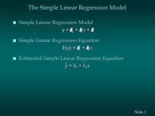
Problems in Applying the Linear Regression Model

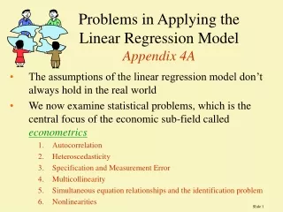
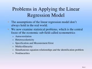
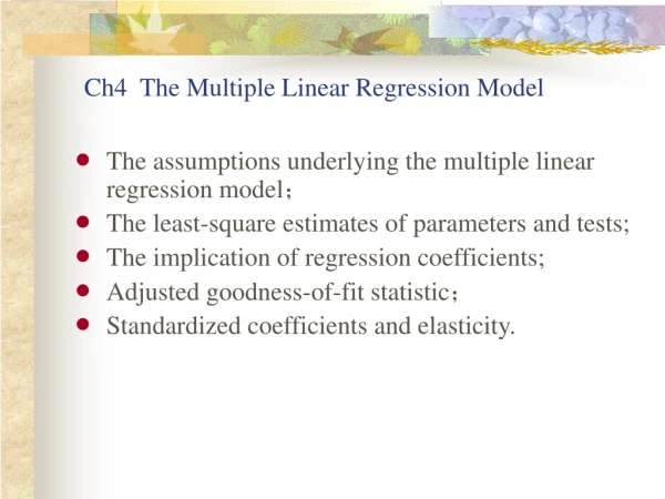
1. Problems in Applying the Linear Regression Model • The assumptions of the linear regression model don’t always hold in the real world. • We now examine statistical problems, which is the central focus of the economic sub-field called econometrics • Autocorrelation • Heteroscedasticity • Specification and Measurement Error • Multicollinearity • Simultaneous equation relationships and the identification problem • Nonlinearities

2. 1. Autocorrelation (serial correlation) • Problem: • Coefficients are unbiased • but t-values are unreliable • Symptoms: • look at a scatter of the error terms to see if there is a pattern, or • check if Durbin Watson statistic is far from 2. • Cures: • Find more variables that explain these patterns • Take first differences of data: Q = α+ β•P

3. Scatter of Error TermsPositive Autocorrelation Y 1 2 6 3 4 5 7 8 X

4. 2. Heteroscedasticity • Problem: • Coefficients are unbiased • t-values are unreliable • Symptoms: • different variances for different sub-samples • scatter of error terms shows increasing or decreasing dispersion • Cures: • Transform data, e.g., transform them into logs • Take averages of each sub-sample and use weighted least squares

5. Scatter of Error TermsHeteroscedasticity Height alternative log Ht = α+β•AGE 1 2 5 8 AGE

6. 3. Specification & Measurement Error • Salary = α + β (Strike Outs) in baseball • we find thatβ is positive !!! • Why? • Omitted variable which is the number of Hits • Salary = c + d (Strike Outs) + e ( Hits ) • here d is negative and e is positive

7. Specification & Measurement Error • Problem: • Coefficients are biased – we can even have the wrong sign as in the baseball example • Even adding more observations will not cure this bias • Symptoms: • The results don’t make economic sense • Cure: • Think through the relationships and find the missing variables in the specification • See if the new specification improves the fit (higher R2) and makes economic sense.

8. Sometimes independent variables aren’t independent. EXAMPLE: Let Q = Eggs sold Q = a + b Pd + c Pg where Pd is price for a dozen eggs and Pg is the price for a gross of eggs. Regression Output Q = 22 - 7.8 Pd -.9 Pg (1.2) (1.45) R-square = .87 (t-values in parentheses) N = 100 observations Notice that: R-square is 87% But that neither coefficient is statistically significant. 4. Multicollinearity

9. Multicollinearity • Problem: • Coefficients are unbiased • The t-values are small, often insignificant • Symptoms: • High R-squares but low t-values • Cures: • Drop a variable. Usually the remaining variable becomes significant. • Do nothing if forecasting, since the added R-square of more variables is worthwhile.

10. 5. Simultaneous Equations and the Identification Problem • Problem: • Coefficients are biased • Symptom: • Independent variables are known to be part of a system of equations (such as Demand and Supply curves) • Cure: • Use as many independent variables as possible.

11. Graphical Explanation of the Identification Problem • Suppose we estimate the following demand curve Q = a + b P. • Suppose Supply varies over the season but Demand is FIXED • For example, you always love strawberries • All points lie on the demand curve • The demand curve is said to be identified. P S1 S2 S3 Demand quantity

12. Suppose instead that SUPPLY is Fixed • Let DEMAND shift and supply is fixed on doesn’t change. • For example, the cost of production of suntan oil doesn’t change, but the demand for it does • All Points are on the SUPPLY curve. • We say that the SUPPLY curve is identified. P Supply D3 D2 D1 quantity

13. When both Supply and Demand Vary P • Often both supply and demand vary. • Equilibrium points are in shaded region. • A regression of Q = a + b Pwill be neither a demand nor a supply curve. S2 S1 ? D2 D1 quantity

14. Simultaneous Systems • Demand is Qd = a + b P + c Y + e1 • Supply is Qs = d + e P + f W + e2 • Where P is price, Y is income, W is the wage rate, and each has an error term. • Notice that P is in both of the demand and supply function. P is “endogenously” determined by both demand and supply. • The simultaneity problem is that price is not independent, as it is determined by the whole system • The cure for this problem is usually to have as many independent variables as possible in the demand regression to make demand act like it is “fixed”.

15. 6. Nonlinear Forms • Semi-logarithmic transformations. Sometimes taking the logarithm of the dependent variable and/or an independent variable improves the R2. Examples are: • lnY = α + ß·X. • Here, Y grows exponentially at rate ß in X; that is, ß percent growth per period. • Y = α + ß·ln X. Here, Y doubles each time X increases by the square of X. ln Y Ln Y = .01 + .05X X

16. Reciprocal Transformations • The relationship between variables may be inverse. Sometimes taking the reciprocal of a variable improves the fit of the regression as in the example: • Y = α + ß·(1/X) • Shapes can be: • declining slowly • if beta positive • rising slowly • if beta negative Y e.g., Y = 500 + 2 ( 1/X) X

17. Polynomials • Quadratic, cubic, and higher degree polynomial relationships are common in business and economics. • Profit and revenue are cubic functions of output. • Average cost is a quadratic function, as it is U-shaped • Total cost is a cubic function, as it is S-shaped • TC = α·Q + ß·Q2 + γ·Q3 is a cubic total cost function. • If higher order polynomials improve the R-square, then the added complexity may be worth it.

18. Multiplicative or Double Log • With the double log form, the coefficients are elasticities • Q = A • P b • Yc • Psd • multiplicative functional form • So: Ln Q = a + b•Ln P + c•Ln Y+ d•Ln Ps • Transform all variables into natural logs • Called the double log, since logs are on the left and the right hand sides. Ln and Log are used interchangeably. We use only natural logs.

19. Soft Drink Case, cross section of 50 states Linear Specification Cans = 515 - 242 Price + 1.19 Income + 2.91Temp Predictor Coeff StDev T P Constant 514.8 113.2 4.55 0.000 Price -241.80 43.65 -5.54 0.000 Income 1.195 1.688 0.71 0.483 Temp 2.9136 0.7071 4.12 0.000 R-Sq = 69.8% R-Sq(adj) = 67.7% The Price elasticity in Wyoming is = (DQ/DP)(P/Q) = -241.8(2.31/102)= -5.476

20. Double Log Soft Drink Case Ln Cans = 2.47 - 3.17 Ln Price + 0.202 Ln Income + 1.12 Ln Temp Predictor Coef Std Dev T P Constant 2.466 1.385 1.78 0.082 Ln Price -3.1695 0.6485 -4.89 0.000 Ln Income 0.2020 0.1834 1.10 0.277 Ln Temp 1.1196 0.2611 4.29 0.000 R-Sq = 67.4% R-Sq(adj) = 65.1% Characterize the demand for soft drinks in the US. Are soft drinks inelastic? Are they luxuries? Which specification fits the data better?