Download

1 / 37
370 likes | 488 Views
This chapter delves into the Indexed Sequential Access Method (ISAM) and highlights its limitations, which motivates the introduction of the B+ Tree structure. We explore the functionality of ISAM, including its index file structure and the binary search method for speeding up data retrieval. By analyzing index sizes, pointers, and the challenges of deletions and insertions, we understand the importance of an optimal indexing mechanism. The chapter also prepares you for upcoming homework and participation opportunities, enhancing your grasp of efficient data management techniques in databases.

E N D
Chapter 9 of DBMS • First we look at a simple (strawman) approach (ISAM). • We will see why it is unsatisfactory. • This will motivate the B+Tree • Read 9.1 to 9.5 • Glance at 9.6 and 9.8.2 • Homework (won’t be graded, but TA’s will be happy to answer questions) 9.1 and 9.2 (with more emphasis on the insertion questions, less on deletion) • For Tuesday glance at chapter 10. • On Thursday Nov 7th, there will be no traditional class. Instead, I will be in my office, and the two TAs will be in the TA Lab, to answer questions during the normal class hours. (We will not have prepared remarks, we will simply answer questions. Participation is optional, the usefulness of the experience depends on you coming in with meaningful questions).
Indexed Sequential Access Method • If our large database is sorted, we can speed up search by doing binary search on the entire database. • However this means we must do log(N) disk accesses… • The idea of ISAM is to do a faster, approximate binary search in main memory, and use this information to do fewer disk accesses (usually only one). :: Data Page 1 Data Page 2 Data Page 3 Data Page N Data Page N-1
KP Maggiepage 7 Indexed Sequential Access Method • An indexentry is a <key,pointer> pair, where key is the value of the first key on the page, and pointer, points to the page. • Example Data Page 7
K1P1 K2P2 K3P3 K3P0 Maggiepage 2 Waylonpage 3 Maggiepage 1 Indexed Sequential Access Method • An indexfile is a concatenation of indexentries. Together with one extra pointer at the beginning. • Example
7 P4 K3P3 Indexed Sequential Access Method Lets look at an indexfile (this one is the smallest possible example) Every record pointed to by this pointer has a value greater that or equal to 7 Every record pointed to by this pointer has a value less that 7
Indexed Sequential Access Method • Instead of doing binary search on the data files, we can do binary search on the index, to find the largest value, which is equal to or less than the search key. We then use the pointer to go to disk to retrieve the relevant block from disk. • Example: we are searching for 8, we do a binary search to find 5, we retrieve page 2, and search it to find a match (if there is one). • Find the largest entry less than the key, follow right child. (find 20) • Find the smallest entry greater than or equal to the key, follow left child. (find 2) Index File 16 :: 5 12 19 p p p p p p Data Files :: Data Page 1 Data Page 2 Data Page 3 Data Page N Data Page N-1
Indexed Sequential Access Method • How big should the index file be? • How about more pointers per page? • We could have two pointers to each page (on average, or exactly). • This does not help, because we have to retrieve a block at a time. Index File 34 :: 2 5 77 p p p p p p Data Files :: Data Page 1 Data Page 2 Data Page 3 Data Page N Data Page N-1
Indexed Sequential Access Method • How big should the index file be? • How about less pointers per page? • We could have a pointer for each two pages (on average, or exactly). • This might help, because it makes the index smaller. We can do a little trick of adding “sideways” pointers. Actually, these “sideways” pointer can be useful for another reason, they can be helpful for range queries. • However, to few pointers leads to chaining…. Index File 16 :: 5 12 19 p p p p p p Data Files :: Data Page 1 Data Page 2 Data Page 3 Data Page N Data Page N-1
Indexed Sequential Access Method • We have seen that too small or too large an index (in other words too few or too many pointers) can be a problem. But suppose the index does not fit in main memory? • The key observation is that the index itself is a sort of database, so lets build an index on the index! 21 p Index File 16 :: 5 12 19 p p p p p p Data Files :: Data Page 1 Data Page 2 Data Page 3 Data Page N Data Page N-1
Tree Based Indexing Data Page 4 Data Page 6 Data Page 8 Data Page 9 Data Page 7 Data Page 5 Data Page 1 Data Page 2 Data Page 3 • An index of indexes is a tree! • We can use this structure to do fast equality search. Find 15, 0 • What about range search? • It looks like we have solved our fast indexing problem, but there is a catch, what happens if we have a deletion, an insertion? Define root internal node leaf 17 14 18 5 13 16 30 35 43 Data Page 10
Tree Based Indexing Over-flow 1 Data Page 6 Data Page 4 Data Page 3 Data Page 8 Data Page 9 Data Page 7 Data Page 1 Data Page 2 Data Page 5 • What happens if we have a deletion? (not much) • What happens if we have an insertion? (trouble!) • Solution: Overflow Buckets • If we have enough overflow buckets, we might as well have no index at all 17 Suppose we add a bunch of 15 year olds to the database… 14 18 5 13 16 30 35 43 Data Page 10
B+-Tree Index Files B+-tree indices are an alternative to indexed-sequential files. • Disadvantage of indexed-sequential files: performance degrades as file grows, since many overflow blocks get created. Periodic reorganization of entire file is required. • Advantage of B+-treeindex files: automatically reorganizes itself with small, local, changes, in the face of insertions and deletions. Reorganization of entire file is not required to maintain performance. • Disadvantage of B+-trees: extra insertion and deletion overhead, space overhead. • Advantages of B+-trees outweigh disadvantages, and they are used extensively.
B+-Tree Index Files (Cont.) A B+-tree is a rooted tree satisfying the following properties: • All paths from root to leaf are of the same length • Let d be the order of the tree (user specified), and let d = n/2 • Each node that is not a root or a leaf has between [n/2] and n children. • A leaf node has between [(n–1)/2] and n–1 values • Special cases: • If the root is not a leaf, it has at least 2 children. • If the root is a leaf (that is, there are no other nodes in the tree), it can have between 0 and (n–1) values.
B+-Tree Node Structure • Typical node • Ki are the search-key values • Pi are pointers to children (for non-leaf nodes) or pointers to records (for leaf nodes). • The fan-out is the number of pointers • The search-keys in a node are ordered K1 < K2 < K3 < . . .< Kn–1
Leaf Nodes in B+-Trees Properties of a leaf node: • For i = 1, 2, . . ., n–1, pointer Pi points to a file record with search-key value Ki. • If Li, Lj are leaf nodes and i < j, Li’s search-key values are less than Lj’s search-key values • Pn points to next leaf node in search-key order
Non-Leaf Nodes in B+-Trees • Non leaf nodes form a multi-level sparse index on the leaf nodes. For a non-leaf node with m pointers: • All the search-keys in the subtree to which P1 points are less than K1 • For 2 i n – 1, all the search-keys in the subtree to which Pi points have values greater than or equal to Ki–1 and less than Km–1 60 5 4.9999.. or less 60.0000 or greater 59.99.. or less
Example of a B+-tree B+-tree for account file (n = 3) • Leaf nodes must have between 1 and 2 values ((n–1)/2 and n –1, with n = 3). • Non-leaf nodes other than root must have between 2 and 3 children ((n/2 and n with n =3). • Root must have at least 2 children.
Example of B+-tree • Leaf nodes must have between 2 and 4 values ((n–1)/2 and n –1, with n = 5). • Non-leaf nodes other than root must have between 3 and 5 children ((n/2 and n with n =5). • Root must have at least 2 children. B+-tree for account file (n = 5)
Observations about B+-trees • Since the inter-node connections are done by pointers, “logically” close blocks need not be “physically” close. • The non-leaf levels of the B+-tree form a hierarchy of sparse indices. • The B+-tree contains a relatively small number of levels (logarithmic in the size of the main file), thus searches can be conducted efficiently. (and a large base logarithm at that) • Insertions and deletions to the main file can be handled efficiently, as the index can be restructured in logarithmic time (as we shall see).
Queries on B+-Trees • Find all records with a search-key value of k. • Start with the root node • Examine the node for the smallest search-key value > k. • If such a value exists, assume it is Kj. Then follow Pi to the child node • Otherwise k Km–1, where there are m pointers in the node. Then follow Pm to the child node. • If the node reached by following the pointer above is not a leaf node, repeat the above procedure on the node, and follow the corresponding pointer. • Eventually reach a leaf node. If for some i, key Ki = k follow pointer Pito the desired record. Else no record with search-key value k exists.
Queries on B+-Trees What is the difference between 5 and 5* ? How come 30 is in the index, but there is no 30* in the file? Find 28*, Find 0*, Find all records > 25 and < 31 Root 17 Entries <= 17 Entries > 17 27 5 13 30 39* 2* 3* 5* 7* 8* 22* 24* 27* 29* 38* 33* 34* 14* 16*
Queries on B+-Trees (Cont.) • In processing a query, a path is traversed in the tree from the root to some leaf node. • If there are K search-key values in the file, the path is no longer than logn/2(K). • A node is generally the same size as a disk block, typically 4 kilobytes, and n is typically around 100 (40 bytes per index entry). • With 1 million search key values and n = 100, at most log50(1,000,000) = 4 nodes are accessed in a lookup. • Contrast this with a balanced binary free with 1 million search key values — around 20 nodes are accessed in a lookup • above difference is significant since every node access may need a disk I/O, costing around 20 milliseconds!
Updates on B+-Trees: Insertion • Find the leaf node in which the search-key value would appear • If the search-key value is already there in the leaf node, record is added to file and if necessary a pointer is inserted into the bucket. • If the search-key value is not there, then add the record to the main file and create a bucket if necessary. Then: • If there is room in the leaf node, insert (key-value, pointer) pair in the leaf node • Otherwise, split the node (along with the new (key-value, pointer) entry) as discussed in the next slide.
13 17 24 30 2* 3* 5* 7* 14* 16* 24* 27* 28* 40* 41* 45* 77* 19* 20* 22* Updates on B+-Trees: Insertion Insert 23 This is the easy case! 13 17 24 30 2* 3* 5* 7* 14* 16* 24* 27* 28* 40* 41* 45* 77* 19* 20* 22* 23*
Updates on B+-Trees: Insertion 13 17 24 30 2* 3* 5* 7* 14* 16* 24* 27* 28* 40* 41* 45* 77* 19* 20* 22* Insert 8 13 17 24 30 5 5* 7* 8* 14* 16* 24* 27* 28* 40* 41* 45* 77* 2* 3* 19* 20* 22* Because the insertion will cause overfill, we split the leaf node into two nodes, we split the data into two nodes (and distribute the data evenly between them). “5” is special, since it discriminates between the two new siblings, so it is copied up. We now need to insert 5 into the parent node…
Updates on B+-Trees: Insertion 13 17 24 30 We now need to insert 5 into the parent node… 5 5* 7* 8* 14* 16* 24* 27* 28* 40* 41* 45* 77* 2* 3* 19* 20* 22* 17 5 13 24 30 5* 7* 8* 14* 16* 24* 27* 28* 40* 41* 45* 77* 2* 3* 19* 20* 22* Because the insertion will cause overfill, we split the node into two nodes, we split the data into two nodes. “17” is special, since it discriminates between the two new siblings, so it is pushed up.
Updates on B+-Trees: Insertion 17 5 13 24 30 5* 7* 8* 14* 16* 24* 27* 28* 40* 41* 45* 77* 2* 3* 19* 20* 22* 17 The insertion of 8 has increased the height of the tree by one (this is rare). 5 13 24 30 5* 7* 8* 14* 16* 24* 27* 28* 40* 41* 45* 77* 2* 3* 19* 20* 22*
Updates on B+-Trees: Insertion (Cont.) • Splitting a node: • take the n(search-key value, pointer) pairs (including the one being inserted) in sorted order. Place the first n/2 in the original node, and the rest in a new node. • let the new node be p, and let k be the least key value in p. Insert (k,p) in the parent of the node being split. If the parent is full, split it and propagate the split further up. • The splitting of nodes proceeds upwards till a node that is not full is found. In the worst case the root node may be split increasing the height of the tree by 1. Result of splitting node containing Brighton and Downtown on inserting Clearview
Updates on B+-Trees: Insertion (Cont.) B+-Tree before and after insertion of “Clearview”
Updates on B+-Trees: Deletion • Find the record to be deleted, and remove it from the main file and from the bucket (if present) • Remove (search-key value, pointer) from the leaf node if there is no bucket or if the bucket has become empty • If the node has too few entries due to the removal, and the entries in the node and a sibling fit into a single node, then • Insert all the search-key values in the two nodes into a single node (the one on the left), and delete the other node. • Delete the pair (Ki–1, Pi), where Pi is the pointer to the deleted node, from its parent, recursively using the above procedure.
Updates on B+-Trees: Deletion • Otherwise, if the node has too few entries due to the removal, and the entries in the node and a sibling fit into a single node, then • Redistribute the pointers between the node and a sibling such that both have more than the minimum number of entries. • Update the corresponding search-key value in the parent of the node. • The node deletions may cascade upwards till a node which has n/2 or more pointers is found. If the root node has only one pointer after deletion, it is deleted and the sole child becomes the root.
Examples of B+-Tree Deletion • The removal of the leaf node containing “Downtown” did not result in its parent having too little pointers. So the cascaded deletions stopped with the deleted leaf node’s parent. Before and after deleting “Downtown”
Examples of B+-Tree Deletion (Cont.) • Node with “Perryridge” becomes underfull (actually empty, in this special case) and merged with its sibling. • As a result “Perryridge” node’s parent became underfull, and was merged with its sibling (and an entry was deleted from their parent) • Root node then had only one child, and was deleted and its child became the new root node Deletion of “Perryridge” from result of previous example
Example of B+-tree Deletion (Cont.) • Parent of leaf containing Perryridge became underfull, and borrowed a pointer from its left sibling • Search-key value in the parent’s parent changes as a result Before and after deletion of “Perryridge” from earlier example
B+-Tree File Optimization • Good space utilization important since records use more space than pointers. • To improve space utilization, involve more sibling nodes in redistribution during splits and merges • Involving 2 siblings in redistribution (to avoid split / merge where possible) results in each node having at least entries Insert 22 13 17 24 30 2* 3* 5* 7* 14* 16* 24* 27* 28* 40* 41* 45* 77* 19* 20* 21* 22*
Indices in SQL CREATE INDEX gpa_ranking ON Students WITH STRUCTURE = BTREE KEY = gpa