Download

1 / 41
410 likes | 581 Views
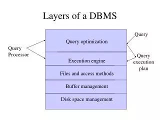
Layers of a DBMS . Query. Query optimization Execution engine Files and access methods Buffer management Disk space management. Query Processor. Query execution plan. The Memory Hierarchy. Main Memory Disk Tape. 5-10 MB/S transmission rates 2-10 GB storage average time to

E N D
Layers of a DBMS Query Query optimization Execution engine Files and access methods Buffer management Disk space management Query Processor Query execution plan
The Memory Hierarchy Main MemoryDisk Tape • 5-10 MB/S • transmission rates • 2-10 GB storage • average time to • access a block: • 10-15 msecs. • Need to consider • seek, rotation, • transfer times. • Keep records “close” • to each other. • 1.5 MB/S transfer rate • 280 GB typical • capacity • Only sequential access • Not for operational • data • Volatile • limited address • spaces • expensive • average access • time: • 10-100 nanoseconds Cache: access time 10 nano’s
Tracks Arm movement Arm assembly Disk Space Manager • Task: manage the location of pages on disk (page = block) • Provides commands for: • allocating and deallocating a page • on disk • reading and writing pages. • Why not use the operating system • for this task? • Portability • Limited size of address space • May need to span several • disk devices. Spindle Disk head Sector Platters
DB Buffer Management in a DBMS Page Requests from Higher Levels • Data must be in RAM for DBMS to operate on it! • Table of <frame#, pageid> pairs is maintained. BUFFER POOL disk page free frame MAIN MEMORY DISK choice of frame dictated by replacement policy
Buffer Manager Manages buffer pool: the pool provides space for a limited number of pages from disk. Needs to decide on page replacement policy. Enables the higher levels of the DBMS to assume that the needed data is in main memory. Why not use the Operating System for the task?? - DBMS may be able to anticipate access patterns - Hence, may also be able to perform prefetching - DBMS needs the ability to force pages to disk.
Record Formats: Fixed Length • Information about field types same for all records in a file; stored in systemcatalogs. • Finding i’th field requires scan of record. • Note the importance of schema information! F3 F4 F1 F2 L3 L4 L1 L2 Address = B+L1+L2 Base address (B)
Files of Records • Page or block is OK when doing I/O, but higher levels of DBMS operate on records, and files of records. • FILE: A collection of pages, each containing a collection of records. Must support: • insert/delete/modify record • read a particular record (specified using record id) • scan all records (possibly with some conditions on the records to be retrieved)
File Organizations • Heap files:Suitable when typical access is a file scan retrieving all records. • Sorted Files:Best if records must be retrieved in some order, or only a `range’ of records is needed. • Hashed Files:Good for equality selections. • File is a collection of buckets. Bucket = primary page plus zero or moreoverflow pages. • Hashing functionh: h(r) = bucket in which record r belongs. h looks at only some of the fields of r, called the search fields.
Cost Model for Our Analysis As a good approximation, we ignore CPU costs: • B: The number of data pages • R: Number of records per page • D: (Average) time to read or write disk page • Measuring number of page I/O’s ignores gains of pre-fetching blocks of pages; thus, even I/O cost is only approximated.
Cost Model for Our Analysis As a good approximation, we ignore CPU costs: • B: The number of data pages • R: Number of records per page • D: (Average) time to read or write disk page • Measuring number of page I/O’s ignores gains of pre-fetching blocks of pages; thus, even I/O cost is only approximated. • Average-case analysis; based on several simplistic assumptions.
Assumptions in Our Analysis • Single record insert and delete. • Heap Files: • Equality selection on key; exactly one match. • Insert always at end of file. • Sorted Files: • Files compacted after deletions. • Selections on sort field(s). • Hashed Files: • No overflow buckets, 80% page occupancy.
Indexes • An index on a file speeds up selections on the search key fields for the index. • Any subset of the fields of a relation can be the search key for an index on the relation. • Search key is not the same as key(minimal set of fields that uniquely identify a record in a relation). • An index contains a collection of data entries, and supports efficient retrieval of all data entries k* with a given key value k.
Alternatives for Data Entry k* in Index • Three alternatives: • Data record with key value k • <k, rid of data record with search key value k> • <k, list of rids of data records with search key k> • Choice of alternative for data entries is orthogonal to the indexing technique used to locate data entries with a given key value k. • Examples of indexing techniques: B+ trees, hash-based structures
Alternatives for Data Entries (2) • Alternative 1: • If this is used, index structure is a file organization for data records (like Heap files or sorted files). • At most one index on a given collection of data records can use Alternative 1. (Otherwise, data records duplicated, leading to redundant storage and potential inconsistency.) • If data records very large, # of pages containing data entries is high. Implies size of auxiliary information in the index is also large, typically.
Alternatives for Data Entries (3) • Alternatives 2 and 3: • Data entries typically much smaller than data records. So, better than Alternative 1 with large data records, especially if search keys are small. • If more than one index is required on a given file, at most one index can use Alternative 1; rest must use Alternatives 2 or 3. • Alternative 3 more compact than Alternative 2, but leads to variable sized data entries even if search keys are of fixed length.
Index Classification • Primary vs. secondary: If search key contains primary key, then called primary index. • Clustered vs. unclustered: If order of data records is the same as, or `close to’, order of data entries, then called clustered index. • Alternative 1 implies clustered, but not vice-versa. • A file can be clustered on at most one search key. • Cost of retrieving data records through index varies greatly based on whether index is clustered or not!
Clustered vs. Unclustered Index Data entries Dataentries (Index File) (Data file) DataRecords Data Records CLUSTERED UNCLUSTERED
Index Classification (Contd.) • Dense vs. Sparse: If there is at least one data entry per search key value (in some data record), then dense. • Alternative 1 always leads to dense index. • Every sparse index is clustered! • Sparse indexes are smaller; Ashby, 25, 3000 22 Basu, 33, 4003 25 Bristow, 30, 2007 30 Ashby 33 Cass, 50, 5004 Cass Smith Daniels, 22, 6003 40 Jones, 40, 6003 44 44 Smith, 44, 3000 50 Tracy, 44, 5004 Sparse Index Dense Index on on Data File Name Age
Index Classification (Contd.) Examples of composite key indexes using lexicographic order. • Composite Search Keys: Search on a combination of fields. • Equality query: Every field value is equal to a constant value. E.g. wrt <sal,age> index: • age=20 and sal =75 • Range query: Some field value is not a constant. E.g.: • age =20; or age=20 and sal > 10 11,80 11 12 12,10 name age sal 12,20 12 13,75 bob 12 10 13 <age, sal> cal 11 80 <age> joe 12 20 10,12 sue 13 75 10 20 20,12 Data records sorted by name 75,13 75 80,11 80 <sal, age> <sal> Data entries in index sorted by <sal,age> Data entries sorted by <sal>
Tree-Based Indexes • ``Find all students with gpa > 3.0’’ • If data is in sorted file, do binary search to find first such student, then scan to find others. • Cost of binary search can be quite high. • Simple idea: Create an `index’ file. Index File kN k2 k1 Data File Page N Page 3 Page 1 Page 2 • Can do binary search on (smaller) index file!
40 51 63 20 33 46* 55* 40* 51* 97* 10* 15* 20* 27* 33* 37* 63* Tree-Based Indexes (2) index entry P K P P K P K m 2 0 1 m 1 2 Root
Index Entries DataEntries B+ Tree: The Most Widely Used Index • Insert/delete at log F N cost; keep tree height-balanced. (F = fanout, N = # leaf pages) • Minimum 50% occupancy (except for root). Each node contains d <= m <= 2d entries. The parameter d is called the order of the tree. Root
Example B+ Tree • Search begins at root, and key comparisons direct it to a leaf. • Search for 5*, 15*, all data entries >= 24* ... 30 24 13 17 39* 22* 24* 27* 38* 3* 5* 19* 20* 29* 33* 34* 2* 7* 14* 16*
B+ Trees in Practice • Typical order: 100. Typical fill-factor: 67%. • average fanout = 133 • Typical capacities: • Height 4: 1334 = 312,900,700 records • Height 3: 1333 = 2,352,637 records • Can often hold top levels in buffer pool: • Level 1 = 1 page = 8 Kbytes • Level 2 = 133 pages = 1 Mbyte • Level 3 = 17,689 pages = 133 MBytes
Inserting a Data Entry into a B+ Tree • Find correct leaf L. • Put data entry onto L. • If L has enough space, done! • Else, must splitL (into L and a new node L2) • Redistribute entries evenly, copy upmiddle key. • Insert index entry pointing to L2 into parent of L. • This can happen recursively • To split index node, redistribute entries evenly, but push upmiddle key. (Contrast with leaf splits.)
Entry to be inserted in parent node. (Note that 17 is pushed up and only 17 this with a leaf split.) 24 30 5 13 Inserting 8* into Example B+ Tree Entry to be inserted in parent node. (Note that 5 is s copied up and • Note: • why minimum occupancy is guaranteed. • Difference between copy-up and push-up. 5 continues to appear in the leaf.) 5* 3* 7* 2* 8* appears once in the index. Contrast
Example B+ Tree After Inserting 8* Root 17 24 30 5 13 39* 2* 3* 19* 20* 22* 24* 27* 38* 5* 7* 8* 29* 33* 34* 14* 16* • Notice that root was split, leading to increase in height. • In this example, we can avoid split by re-distributing entries; however, this is usually not done in practice.
Deleting a Data Entry from a B+ Tree • Start at root, find leaf L where entry belongs. • Remove the entry. • If L is at least half-full, done! • If L has only d-1 entries, • Try to re-distribute, borrowing from sibling (adjacent node with same parent as L). • If re-distribution fails, mergeL and sibling. • If merge occurred, must delete entry (pointing to L or sibling) from parent of L. • Merge could propagate to root, decreasing height.
Example Tree After (Inserting 8*, Then) Deleting 19* and 20* ... • Deleting 19* is easy. • Deleting 20* is done with re-distribution. Notice how middle key is copied up. Root 17 27 30 5 13 39* 2* 3* 22* 24* 27* 29* 38* 5* 7* 8* 33* 34* 14* 16*
... And Then Deleting 24* • Must merge. • Observe `toss’ of index entry (on right), and `pull down’ of index entry (below). 30 39* 22* 27* 38* 29* 33* 34* 5 13 17 30 39* 3* 22* 38* 2* 5* 7* 8* 27* 33* 34* 29* 14* 16*
Multidimensional Indexes • Applications: geographical databases, data cubes. • Types of queries: • partial match (give only a subset of the dimensions) • range queries • nearest neighbor • Where am I? (DB or not DB?) • Conventional indexes don’t work well here.
Indexing Techniques • Hash like structures: • Grid files • Partitioned indexing functions • Tree like structures: • Multiple key indexes • kd-trees • Quad trees • R-trees
Grid Files • Each region in the file • corresponds to a • bucket. • Works well even if • we only have partial • matches • Some buckets may • be empty. • Reorganization requires • moving grid lines. • Number of buckets • grows exponentially • with the dimensions. 500K * * * * * * * 250K * * 200K * 90K * Salary * * * * 10K * 0 15 20 35 102 Age
Partitioned Hash Functions • A hash function produces k bits identifying the bucket. • The bits are partitioned among the different attributes. • Example: • Age produces the first 3 bits of the bucket number. • Salary produces the last 3 bits. • Supports partial matches, but is useless for range queries.
Tree Based Indexing Techniques Salary, 150 Age, 60 Age, 47 70, 110 Salary, 300 85, 140 * * * * * * * * * * * * *
Multiple Key Indexes • Each level as an index for one • of the attributes. • Works well for partial matches • if the match includes the first • attributes. Index on first attribute Index on second attribute
Adaptation to secondary storage: KD Trees • Allow multiway branches • at the nodes, or • Group interior nodes • into blocks. Salary, 150 Age, 60 Age, 47 50, 275 70, 110 Salary, 80 Salary, 300 60, 260 85, 140 50, 100 Age, 38 50, 120 30, 260 25, 400 25, 60 45, 60 45, 350 50, 75
Quad Trees • Each interior node corresponds • to a square region (or k-dimen) • When there are too many points • in the region to fit into a block, • split it in 4. • Access algorithms similar to those • of KD-trees. 400K * * * * * * * * * * * Salary * * 0 100 Age
R-Trees • Interior nodes contain sets • of regions. • Regions can overlap and not • cover all parent’s region. • Typical query: • Where am I? • Can be used to store regions • as well as data points. • Inserting a new region may • involve extending one of the • existing regions (minimally). • Splitting leaves is also tricky.