Finite Settling Time Design
Finite Settling Time Design. Outline. • Finite settling for DT systems. • Finite settling time controllers. • Deadbeat controllers. • Example. • Inter-sample behavior. Finite Settling Time. • CT systems: asymptotically (infinite time) settle at the desired output.


Finite Settling Time Design
E N D
Presentation Transcript
Outline • Finite settling for DT systems. • Finite settling time controllers. • Deadbeat controllers. • Example. • Inter-sample behavior.
Finite Settling Time • CT systems: asymptotically (infinite time) settle at the desired output. • DT systems: can settle at the reference output after a finite interval then follow it exactly. • Finite settling time designs may exhibit undesirable inter-sample behavior and must be carefully checked before implementation. • Use a synthesis approach to obtain the desired controller for finite settling time.
Reference Input • Examine the general z-transform of a standard reference input.
Select Error • Assume zero error after m sampling periods and the error = N(z) • Thus, a unit step must be tracked perfectly starting at the first sampling point, a ramp at the second, and so on.
Controller • Solve for the controller C(z)
Dead beat control • In discrete-time, the dead beat control problem consists of finding what input signal must be applied to a system in order to bring the output to the steady state in the smallest number of time steps. • For an Nth-order linear system it can be shown that this minimum number of steps will be at most N. The solution is to apply feedback such that all poles of the closed-loop transfer function are at the origin of the z-plane. Therefore the linear case is easy to solve. By extension, a closed loop transfer function which has all poles of the transfer function at the origin is sometimes called a dead beat transfer function
The deadbeat response has the following characteristics • Zero steady-state error. • Minimum rise time. • Minimum settling time. • Less than 2% overshoot/undershoot
Deadbeat Controller • Zeros of the transfer function become poles of the controller C(z) unless they cancel with a pole at z = 1. • GZAS(z) zeros must be inside the unit circle.
Example 6.13 Design a deadbeat controller with T = 0.1 s for the 1-D.O.F. robot with unity moment of inertia neglecting gravity and friction.
System Model Equation of motion (neglect gravity and friction) Plant transfer function z-transfer function of plant, DAC, ADC
Deadbeat Control Large gain may saturate DAC. • Controller causes inter-sample oscillations. • Controller is much worse than the error at the sampling points would indicate.
Block diagram for finite settling timedesign with analog output.
Analog Output • Use transfer function of ZOH. • Use block diagram manipulation.
Limitations of deadbeat control 1- Minimum phase transfer function GZAS(z) (i.e. all zeros inside the unit circle), since its zeros are controller poles. 2-Controller may require excessively high gains that cause DAC saturation. 3-Intersample oscillations of system analog output. Lesson from finite settling time designs: Check analog output of digital control system for satisfactory intersample behavior.
HW # 5 P. 6.6, P 6.8, P 6.13