Download
1 / 19
190 likes | 379 Views
Applying Sequential, Sparse Gaussian Processes – an Illustration Based on SIC2004. Ben Ingram Neural Computing Research Group Aston University, Birmingham, UK. Spatial Interpolation Comparison 2004. What is SIC2004? SIC2004 objectives are to: generate results that are reliable

E N D
Applying Sequential, Sparse Gaussian Processes – an Illustration Based on SIC2004 Ben Ingram Neural Computing Research Group Aston University, Birmingham, UK
Spatial Interpolation Comparison 2004 • What is SIC2004? • SIC2004 objectives are to: • generate results that are reliable • generate results in smallest amount of time • generate results automatically • deal with anomalies • Data provided: background gamma radiation in Germany
Spatial Interpolation Comparison 2004 • Radiation data from 10 randomly selected days were given to participants to devise a method that met the criteria of SIC2004 • For each day there were 200 observations made at the locations shown by red circles • The aim: to predict as fast and as accurately as possible at 808 locations (black crosses) given 200 observations for an 11th randomly selected day
Sequential Sparse Gaussian Processes • Gaussian processes equivalent to Kriging [Cornford 2002] • SSGP use a subset of the dataset called ‘basis vectors’ to best approximate the Gaussian process • Traditional methods require a matrix inversion which is n3 operation, nm2 (where m is number of ‘basis vectors’) • Model complexity controlled by ‘basis vectors’, but important features in the data retained
Sequential Sparse Gaussian Processes • Bayesian Approach • Utilizes prior knowledge such as experience, expert knowledge or previous datasets • Model parameters described by Prior probability distribution • Likelihood: how likely is it that the parameters w generated the data D • Posterior distribution of parameters proportional to product of the likelihood and prior Likelihood Prior Posterior Bayes rule Normalising constant
Choosing Model for SSGP • Machine Learning community treat estimating the covariance function differently • In Geostatistics experiment variogram computed and an appropriate model fitted • In Machine Learning the model is chosen based on experience or informed intuition • How could the 10 prior datasets be used? • Assume data is independent but identically distributed • Compute experimental variograms for subset of data (160 observations) for 10 prior days • Fitted various variogram models and used them in cross-validation for predicting at the 40 withheld locations
Variography • Several models were fitted including mixtures of models variance lag distance • Mixture model consistently fitted better
Variography • Experimental variogram used to select covariance model for SSGP • Insufficient number of observations at smaller lag distances to learn behaviour • Assume little variation at short separation distances • Use tighter variance with hyper-parameters of squared exponential component
Boosting • Boosting used to estimate ‘best’ hyper-parameters (nugget, sill and range) • Adjust the hyper-parameters to maximize the likelihood of the training data • Iterative method used to search for optimal values of the hyper-parameters • Boosting assumes that each iterative step to locate the optimal hyper-parameters is composed of a linear combination of the individual iterative steps calculated for each day • Leave-one-out cross-validation used • 9 days used to estimate optimal parameters • Used resulting hyper-parameters as mean value for hyper-parameters to on left out dataset • Some information about hyper-parameters learnt, but the values are not fixed. Differing degrees of uncertainty associated with each hyper-parameter
Interpolating using SSGP • Anisotropic covariance functions were used because we believed that the variation was not uniform in all directions • Learnt hyper-parameters used to set initial hyper-parameter values for SSGP • How were the number of ‘basis vectors’ (model complexity) chosen? • Cross-validation • Accuracy decreases as number of ‘basis vectors’ decreases
Using our method with the competition data • SSGP was used with 11th day dataset to predict at 808 locations • In addition to the data for the 11th day a “joker” dataset was given • ‘Joker’ dataset simulated a radiation leak into the environment – but contestants did not know this until after the contest • SSGP was used with ‘joker’ dataset to predict at the same 808 locations
Results • To determine how well SSGP performed, we compared it with some standard Machine learning techniques: • Multi-layer perceptrons • Radial basis functions • Gaussian processes • Netlab Matlab toolbox was used for calculations
Contour Maps SSGP GP Actual
Contour Maps - Joker SSGP GP Actual
Learnt hyper-parameters • Exponential range parameters break down as noise parameter becomes large • Squared Exponential parameters relatively constant between datasets
Conclusions • Once nature of covariance structure is understood, interpolation with SSGP is completely automatic • There were problems predicting when there were extreme values, this would be expected • Incorporating a robust estimation method for data with anomalies should be investigated • For 11th day dataset SSGP and GP produced similar results, but SSGP is faster • SSGP devised for large datasets, but can improve speed with small datasets.
Acknowledgements • Lehel Csato – Developer of SSGP algorithm SSGP software available from: http://www.ncrg.aston.ac.uk