Long Range Dependent Traffic and Leaky Buckets
200 likes | 404 Views
Long Range Dependent Traffic and Leaky Buckets. CS215-winter ’01 Demetrios Laios 3/22/2001. Describes the behavior of data source.

Long Range Dependent Traffic and Leaky Buckets
E N D
Presentation Transcript
Long Range Dependent Traffic and Leaky Buckets CS215-winter ’01 Demetrios Laios 3/22/2001
Describes the behavior of data source • A necessary component of a good queueing-system model is an arrival-process model that reflects behavior of the actual arrival process sufficiently closely to explain and/or predict the effect of the arrival process on the system • Informative descriptors of arrival processes • The objective of policing policies such as a leaky-bucket scheme is to reduce congestion by restricting the burstiness of the arrival process.
Burstiness • is roughly, the tendency of arrivals to occur in clusters, or bursts, separated by periods of relatively few arrivals, has become commonplace. • The significance of burstiness is that it has a pronounced adverse effect on queueing-system behavior. • For example, a bursty arrival stream may cause the system to undergo excursions into periods of severe congestion. • Various descriptors of traffic processes can be found in the literature.
Linear Bounded Arrival Processes (LBAP)The use of bounded burstiness inputs has been introduced by Cruz (1987) • AN LBAP-constrained source bounds the number of bits it transmits in any interval of length by a linear function of t. Number of bits transmitted in any interval of length + b • is roughly the long-term average rate allocated by the net to the source and • b is the maximum burst may sent given the choice of • Leaky bucket scheme regulates a LBAP source • Count is incremented by 1 every 1/ seconds, up to a maximum of b
LBAP Cont. • Leaky bucket analogy • packets waiting for a permit • one permit added every 1/ seconds • packets with permits awaiting transmission • holds only b permits • The bucket size b is an important parameter in determining the effectiveness of the leaky bucket scheme • Small b delays bursty traffic • Large b can lead to downstream congestion and buffer overflow
The Leaky Bucket Scheme transmission tokens i token bucket size bi output connection i data buffer leaky bucket enforces Ai(t1,t2) bi + i (t2-t1)
Properties of Leaky Bucket • can thing of this as a single-server queueing system with constant service rate • can act as • peak rate if = peak rate, b = 1 • or moving-window average rate regulator if = avg rate, b = 1 • can act as policer (no packet buffer) • Allows to sent a maximun number of packets given the bucketatthe max bit rate • Performance (loss rate) depends only on the sum of the packet buffer size and the token bucket size (one trades off other exactly)
Traffic bounds • The model bounds the traffic (rather than exactly characterize) • Several different bounds can be obtained for any traffic source (in the same model): • trade off: token bucket size (b value) against bandwidth share ( value) • More bucket depth: larger (worst-case) delays; more jitter • More bandwidth: lower overall utilization; future connections more likely to be rejected
b (, b)=0 Knee point K1 P A K2 Choosing LBAP parameters A, average rate P, peak rate If b slightly < K1 increase If slightly < K2 b is larger
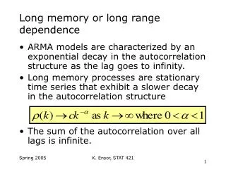
Long-memory (self similar) model • Studies show that packet traffic is strongly auto-correlated and there exists a long-range dependency (LRD), i.e. persistence in their correlation structured does not die even for large lags. • Suppose X, second order (weak or covariance or wide-sense) stationary stochastic process • mean = E[Xt] • variance E[(Xt- )2] = 0 • autocovariance k = E[(Xt- ) (Xt+k- )], k = 0, 1,.., k= k/ 0 • Short-range dependence, or process with short memory or short range correlations or weak dependence • SRD: k k < • Long-range dependence, or process with long memory or long range correlations or strong dependence • LRD: k k i.e. diverges
Shuffling the time series of original traffic traceTransform the original traffic trace, preserving the marginal distribution, peak, average rate while destroying correlations • External shuffle: • Divide the original sequence into blocks of size M. With n data times, there are n/M such blocks. • Then,while preserving the sequence inside each block, the order of blocks is shuffled • Effect:destroying the long-range correlations in data, while preserving the short-range correlations • Internal shuffle: • Now, while preserving the sequence of blocks, a sequence of interarrival times inside each block, is shuffled. • Effect:destroying the short-range correlations in data, while preserving the long-range correlations • Total shuffling:destroy short and long range correlation
Statistical bound • P[A(t1,t2) (t2- t1) + b] <= const where A(t1,t2) is written in terms of Fractional Brownian motion A(t, ) = m + BH(t + ) - BH(t)=dm + BH(), = t2- t1 H : Hurst parameter m : average source bit rate • Applying Large Deviations Techniques we get the following form of LBAP curve (,b)=0, (,b) = A(, H)( -m)2H- b 2-2H where, A(, H) = [2 2H 2H(1-H)2-2H]-1
Network Power • A measure of the efficiency of the congestion control scheme • Power = (Throughput)a /delay • Chose the exponent a based on the relative emphasis placed on throughput versus delay: • if throughput is more important, then a value of a greater than one is chosen. • if throughput and delay are equally important, then a equal to one is chosen. • Clearly, we wish to have lots of throughput and small delay. Unfortunately, these cannot both be achieved simultaneously, and so we are looking for the “operating point” for the system.
Design problem(work in progress) • Maximize power f (,b) = 2/b • Such that: • LBAP curve : (,b) = A(,H)(-m)2H- b2-2H = 0 where, A(,H) = [2 2H 2H(1-H)2-2H]-1 Gives (?): *= m[1- 2H]-1 b* =
Design problem • We have the figure LBAP curve b power
Aggregated TCP flows(work in progess) • TCP remains the dominant traffic protocol through all hours of the day. • TCP traffic typically contributes over 95% of the total traffic volume (UDP protocol at about 2-5% ). • A mixture of both well-known applications (http, ftp, smtp, nntp) (70-80% of the total traffic volume), and less known, contribute significan portions to the TCP traffic mix. • Available trace files http://moat.nlanr.net/Traces/ (NLANR: National Laboratory for Networking Traffic)
Aggregated TCP flows, Cont. • Friendly TCP Traffic for Differentiated Services; • TCP shaping is effective tool for managing TCP traffic; • to decrease the burstiness of UDP and TCP traffic, thereby decreasing the load on the router and switch buffers as well as the latency jitter caused by long queues. • The bursts are spread out over time rather than occur at one time. • Each source is at a higher congestion window when the first drop for that particular source occurs as compared to the case of without shaping. Consequently each source gets a higher throughput and higher goodput (also a higher number of drops). The link utilization is better in this case since all sources do not cut down at around the same instant but rather the drops are spread out over time.
Many thanks to Gregorio Procissi