Advanced Radio Telescope Systems for Precision Astronomy
Explore the goals, arrays, and performance factors of radio telescopes for improved sensitivity and source isolation. Learn about Long Baseline Arrays, European VLBI Network, and high-redshift quasars. Discover how to measure intensities, compute noise levels, and enhance observation capabilities through spatial frequency content analysis.

Advanced Radio Telescope Systems for Precision Astronomy
E N D
Presentation Transcript
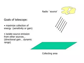
Radio `source’ • Goals of telescope: • maximize collection of energy (sensitivity or gain) • isolate source emission from other sources… (directional gain… dynamic range) Collecting area
LBA: Long Baseline Array in AU EVN: European VLBI Network(more and bigger dishes than VLBA)
Example 3: Array High redshift quasar with continuum flux density Sn = 1 mJy (Ta = SnAeff /2k) Ka = Ta / Sn = Aeff /2k [K/Jy] = 0.7 K/JyParkes = 6 x 0.1 = 0.6 K/JyACTA rms = DS = (fac)(Tsys /Ka)/(B tint)1/2 ATCA (B=128 MHz): 1 mJy = 5 rmsmeans DS= 0.2 mJy rms = DS = (fac)(Tsys /Ka)/(B tint)1/2 = (1.4)(30/0.6)/(B tint)1/2 tint= (70/0.0002)2/(128x106) ~16 min
ARRAYS: Sensivity depends on collecting area Angular resolution ~ l/D D
Example 3: Array High redshift quasar with continuum flux density Sn = 1 mJy (Ta = SnAeff /2k) Ka = Ta / Sn = Aeff /2k [K/Jy] = 0.7 K/JyParkes = 6 x 0.1 = 0.6 K/JyACTA rms = DS = (fac)(Tsys /Ka)/(B tint)1/2 ATCA (B=128 MHz): 1 mJy = 5 rmsmeans DS= 0.2 mJy rms = DS = (fac)(Tsys /Ka)/(B tint)1/2 = (1.4)(30/0.6)/(B tint)1/2 tint= (70/0.0002)2/(128x106) ~16 min
Sensivity depends on collecting area Angular resolution ~ l/D D
Maps from Arrays (or Aperture Synthesis Telescopes): • intensities indicated in ‘units’ of `milli-Jansky per beam’ [why?] • can compute noise level sJy using radiometer equation • can compute beam size from Q ~l/D so W ~ pQ2/4 sterad • best to think of ‘mJy/beam’ as Intensity, In = 2kTB/l2 • then, uncertainty is DTB ~ sJy /W • IMPORTANT: lose surface brightness sensitivity when dilute the • aperture by separating the array telescopes !!! • Hurts ability to see diffuse emission.
Source Strength Angle Fourier Transform Effect of observing complex source with a ‘beam’ Zoom of FT
view convolution of source with beam as filtering in the Spatial Frequency Domain Fourier Transform Zoom of FT Filter
The `microwave sky’ (all sky picture from WMAP map.gfsc.nasa.gov) Example of importance of Spatial Frequency Content
L = 50 (spatial frequency)
Interference Fringes and “Visibility” …. (Visibilities) The term “visibility” has its origin in optical interferometry, where fringes of unresolved sources has high “fringe visibility.” The term “visibilities” in radio astronomy generally refer to a set of measurements of the visibility function of a celestial source.
Simple cross correlation radio interferometer: on-axis source
M Radio `source’ L Interferometer Response Angle, Q • Consider: • ‘point source’ response … full amplitude, but fringe ambiguity • ‘resolved source’ response … source fills + and – fringes => signal • cancels and response -> 0.
The fringe spacing and orientation corresponding to a single ‘u-v’ point:
U-V sampling comes from forming interferometers among all pairs of telescopes in the array: Locations on Earth Instantaneous UV Coverage Earth rotation
See:www.narrabri.atnf.csiro.au/astronomy/vri.html to access the Virtual Radio Interferometer simulator.