Download
1 / 1
10 likes | 139 Views
Exposed Facility. MAXI will be here. GSC counter. Anode direction. Position sensitivity is along with the anode direction. θ col. X-ray. X-ray. φ col. Slit. top. y i (top). mid. bot. slat. Counter. y i (mid) (φ col ). slat. y 63 (bot) (φ col ). y 62 (bot) (φ col ).

E N D
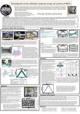
Exposed Facility MAXI will be here. GSC counter Anode direction Position sensitivity is along with the anode direction. θcol X-ray X-ray φcol Slit top y i (top) mid bot slat Counter y i (mid) (φcol) slat y63(bot) (φcol) y62(bot) (φcol) y i (bot) (φcol) y 2(bot) (φcol) y 1(bot) (φcol) y 0(bot) (φcol) Sash Beryllium Window θ = -1.1 deg θ = -0.4 deg θ = 0.0 deg θ = 0.4 deg θ = 1.1 deg Development of the collimator response of gas slit camera of MAXI Mikio Moriia, Masaru Matsuokaa, Shiro Uenoa, Hiroshi Tomidaa, Haruyoshi Katayamaa, Kazuyoshi Kawasakia, Takao Yokotaa, Naoyuki Kuramataa, Tatehiro Miharab, Mitsuhiro Kohamab, Naoki Isobeb, Motoki Nakajimab, Hiroshi Tsunemic, Emi Miyatac, Atsumasa Yoshidad, Kazutaka Yamaokad, Yuichiro Tsuchiyad, Takehiro Miyakawad, Nobuyuki Kawaie, Jun Kataokae, Satoshi Tanakae and Hiroshi Negorof aJapan Aerospace Exploration Agency (JAXA), bRIKEN (The Institute of Physical and Chemical Research), cDepartment of Earth and Space Science, Osaka University, dDepartment of Physics and Mathmatics, Aoyama Gakuin University, eDepartment of Physics, Tokyo Institute of Technology, fDepartment of Physics, Nihon University Home page: http://www-maxi.tksc.jaxa.jp/ Appearance of MAXI (Thermal Technical Model) Abstract Monitor of All-sky X-ray Image (MAXI) is an X-ray all-sky scanner, which will be attached on Exposed Facility of Japanese Experiment Module dubbed "Kibo“ of International Space Station (ISS). MAXI will be launched by the Space Shuttle or the Japanese H-IIA Transfer Vehicle (HTV) in 2008 (ref 1 – 3). MAXI carries two types of X-ray cameras: Solid-state Slit Camera (SSC)(ref. 4, 5) for 0.5 – 10 keV and Gas Slit Camera (GSC) (ref. 6, 7) for 2 – 30 keV bands. Both have long narrow fields of view (FOV) made by a slit and orthogonally arranged collimator plates (slats). The FOV will sweep almost the whole sky once every 96 minutes by utilizing the orbital motion of ISS. Then the light curve of an X-ray point source become triangular shape in one transit. In this paper, we present the actual triangular response of the GSC collimator, obtained by our calibration. In fact they are deformed by gaps between the slats, leaning angle of the slats, and the effective width of the slats. We are measuring these sizes by shooting X-ray beams into the detector behind the collimator. We summarize the calibration and present the first compilation of the data to make the GSC collimator response, which will be useful for public users. Introduction: MAXI, GSC and collimator Results of Calibration Structure of MAXI X-scan International Space Station (ISS) • The actual characteristic of the effective length • revealed by X-scan is as follows: • The peak of the triangular function become rounded off (Figure 7, left). • The bottom ends of the triangular function trail their skirts (Figure 7, left). • The peaks of the triangular function (Δθ) vary with φ(Figure 7, right). Solid-state Slit Camera Figure 7. (left) An example of the effective length Leff as a function of θmeasured by our X-scan. The solid line shows an ideal function Leff (θ). The residual of the data from the ideal function is plotted in the lower panel. The ideal function was fit to minimize the sum of the residuals, varying the peak position of the triangular function (Δθ) as a free parameter. (right) The dependence of the Δθparameter (the left figure) on φmeasured by our X-scan calibration. The upward-sloping curves are caused by the ~0.1 (deg) rotation of a GSCU around the axis of the X-ray beam direction. Japanese Experiment Module (Kibo) Gas Slit Camera Figure 1. MAXI is an all-sky X-ray monitor, which will be attached on Exposed Facility of Japanese Experiment Module “Kibo” of International Space Station (ISS). MAXI carries Gas Slit Camera (GSC) (for 2 – 30 keV) and Solid-state Slit Camera (SSC) (for 0.5 – 10 keV). GSC and SSC consist of a collimator assembly and detectors. The detectors of GSC and SSC are gas proportional counters with one-dimensional position sensitivity and X-ray CCDs operated in the mode with one-dimensional position sensitivity. Z-scan The effective slit width dslit (eff) obtained by Z-scan can be fit well by dslit (eff) = dslit cos( φ – Δφ) (Eq. 1). We found the following characteristic: iv. Slit width (dslit) is not constant along with the slit direction. v. Δφ is not 0 (deg) due to leaning angle of Z-stage and the difference between the edge heights of two tungsten plates (Figure 8, right). The latter is caused by the fact that the two tungsten plates are attached at a slant on the peak of a GSCU. GSC Unit and Field of View Figure 2. Two GSC counters (left figure) and a collimator assembly constitute a GSC Unit (GSCU) (right figure). The collimator assembly is composed of a slit and equally narrow-spaced thin plates (It is also called slats or sheets.) which are arranged orthogonally to the slit, those making fan-like long narrow field of view (FOV). One-dimensional position sensitivity of GSC counters are along with the slats. Therefore, the angle φ (right figure) in the FOV can be measured. A GSCU has FOV of 3 deg (θ) × 80 deg (φ). A collimator assembly is made up of two pairs of a slit and 64 collimator sheets, beneath which counters are aligned. A slit is made up of two edges of tungsten plates attached at a slant on the peak of a GSCU. Figure 8. (left) The dependence of the effective slit width (dslit (eff) ) on the φ. It can be fit well by the equation (1). (Right) The dslit (the top panel) and Δφ(the middle panel) for the positions above every anode wires (C0, C1, ..., C5) obtained by the analysis shown in the left figure. The difference between the edge heights of two tungsten plates (the bottom panel) are derived by dslit × cos (Δφ). FOVs of MAXI GSC Response Figure3. Three GSCUs are assembled and arranged so that FOVs can orient to the horizontal or zenith direction with respect to the ISS motion (Figure 1, left). This GSCU assembly is called GSC-H or GSC-Z camera. These perpendicular FOVs of H and Z cameras are complementary to scan the all-sky during one ISS orbit (96 min.) in spite of shutdowns of detectors when ISS passes through high particle background regions such as South Atlantic Anomaly (SAA). Thanks to ISS motion orbiting around Earth, the angle θin the FOV can be measured for the celestial sphere, roughly by the time when the FOV sweeps an X-ray source, and precisely by a triangular light curve during a transit of the source. We are developing a detector response matrix (DRM) builder (ref. 8), a software to make DRM for each GSCU with given angles (θ, φ) of incident X-rays. The geometry of the collimator assembly estimated by our calibration was incorporated in a collimator function in this DRM builder as follows: • The tungsten slit edge positions (the edge heights and widths between two edges): These positions were obtained by Z-scan. • The list of the positions of the top and bottom edges of 64 sheets: • y i (top) (i = 0,1, ..., 64) and • y i(bot) (φ) (i = 0,1, ..., 64). • These lists were obtained by X-scan light curves, analyzing the times of the edges. We use different lists of the bottom edges for every φ,because the position of the bottom edges of the sheets depend on φof incident X-rays. The top and bottom lists represents the condition that 64 sheets lean in various angles in θdirection. • 3. The list of the minimum effective slat width: This is determined by the width of the dip in X-scan light curve. The minimum of these values with respect to θrepresent the curvature as shown in Figure 9.We simplified the slat shape by dogleg shape (in other words, “く“ • Ku-no-ji in Japanese), because it was difficult to estimate actual shapes of the sheets. Figure 4. The effective area of the collimator depends only on the angle of incident X-rays (θ, φ). The effective area (Seff) of the i-th space between two collimator sheets is calculated as shown in the left figure. Right figure shows triangular shapes of the function Seff . For the purpose of calibration, we define effective length Leff as Seff = L eff× dslit × cos φ Figure 9. The model of geometry incorporated in our collimator response function. This function judge whether the incident photon hits at a slit, slats, and sashes, or not. The slit positions, yi(top) , yi(bot)(φ), and yi(mid)(φ) obtained by our calibration were used in this function. The left-top figure shows the cross sectional view of a GSCU. The left-bottom and right figure shows the images viewed from the directions of the corresponding large arrows. Table 1. Specification of a collimator assembly. Calibration Figure 10. An example of the triangle function Leff measured by our X-scan calibration (points). The solid line shows an simulated function, which could reproduce the actual data to a certain degree. However, there are somewhat difference between the data and model. It is also remaining problem to find some good function to interpolate φ dependence of the functions yi(bot)(φ) and yi(mid)(φ), because we obtained these lists only for some φ values. It is necessary to measure the actual effective area Seff for the entire FOV: -1.5 < θ< 1.5, -40 < φ< 40. Especially, the θdependence is important, because the shape of the light curve of an X-ray source is nearly equal to Seff (θ) thanks to ISS motion (Figure 3). We performed calibration of GSC collimator assemblies of flight model in Tsukuba Space Center of JAXA. The setup of our calibration is shown in Figure 5. We performed two types of operation: X-scan and Z-scan. In X-scan, we changed θin some steps from -1.7 (deg) to 1.7 (deg). For everyθ, we slide the GSCU along with the X_stage axis, passing the X-ray beam through the center of the slit. Figure 6 shows examples of the light curves of X-scan, from which we can measure the effective length L eff . Figure 7 shows an example of measured L eff (θ) in comparison with the ideal function. In Z-scan, we set θ = 0 (deg). For positions around centers of six anode wires, we slide the GSCU along with the Z_stage axis to transverse the slit. From the Z-scan light curve, we can measure the effective slit width dslit (eff) in the φ. Figure 8 shows an example of the dslit (eff) as a function of φ. Conclusion and Prospect We showed the status of development for the collimator response of GSCU of MAXI. We showed our modeling could reproduce the actual response measured by our collimator calibration to a certain degree. However, there are somewhat remaining difference between the data and the simulation. We will attempt to solve this problem. Besides, it was the result only for a counter in the first GSCU of flight model for some φ values. We will apply and check this method to all GSCU of flight model (FM1 -- FM6). These collimator responses will be used as actual response in orbit at the early phase. Nonetheless, it is predicted that the collimator response in orbit would change from that obtained in the ground calibration due to intense vibration at the launch and microgravity. In fact, we learned that the collimator sheets were slightly curved after vibration tests. This curve would change the lists yi(top) , yi(bot)(φ), and yi(mid)(φ). We will randomize these lists around the ground calibration values to fit the orbital data. The response will be refined in this way after accumulating the photon statistic months or years later. Figure 5. Setup of our collimator calibration. Figure 6. Examples of light curves obtained by our X-scan calibration. The narrow or wide dips made by shadows of collimator sheets or of sashes of a GSC counter are clearly seen in the middle panel (θ = 0.0 deg). The interval between a dip to dip gives effective length L eff . Reference • M. Matsuoka, et al., Proc. SPIE, 3114, p414, (1997) • H. Tomida, et al., Proc. SPIE, 4012, p178, (2000) • S. Ueno, et al., Proc. SPIE, 5488, p197, (2004) • H. Katayama, et al., Proc. SPIE, 5501, p1, (2004) 5. E. Miyata, et al., Proc. SPIE, 5165, p366, (2004) 6. T. Mihara, et al., Proc. SPIE, 4497, p173, (2002) 7. N. Isobe, et al., Proc. SPIE, 5165, p354, (2004) 8. Y. Tsuchiya, et al., Proc. SPIE, 5898, p403, (2005) The times of the edges give the position of yi(top) and yi(bot)(φ) (see “Response”). The minimum width of the dip made by the collimator sheets around θ = 0.0 (deg) indicates the effective width of the collimator sheets (see “Response”).