Download
1 / 27
510 likes | 1.69k Views
Precipitation – Gauge Network. Precipitation varies both in time and space Sound hydrologic/hydraulic designs require adequate estimation of temporal/ spatial precipitation patterns. The density of rain gauge network depends on (1) purpose of the study;

E N D
Precipitation – Gauge Network • Precipitation varies both in time and space • Sound hydrologic/hydraulic designs require adequate • estimation of temporal/ spatial precipitation patterns. • The density of rain gauge network depends on • (1) purpose of the study; • (2) geographic configuration of the study region; • (3) economic consideration.
Rain Gauge Density in HK Rain gauge density in HK is: · Daily 13.6 km2/gauge · Autographic/ Automatic 11.0 km2/gauge Rain gauge density is significant higher in Hong Kong Island and much sparse relatively in New Territory (see figure).
World Meteorological Organization (WMO) Suggestion A minimum density for precipitation gauge network: (at least 10% are automatic recording gauges) I: Flat region of temperature, Mediterranean & tropical zones; IIa: Mountain region of temperate, Mediterranean & tropical zones IIb: Small mountains island with very irregular precipitation requiring very dense hydrographic network III: Arid and polar zones
Errors Precipitation Measurement 1. Human Error: scale reading & water displacement (if a dip stick is used) 2. Instrumental Defect: water to moisten the gauge; speed at which mechanical devices work (such as tipping bucket gages); & inadequate use of wind shield 3. Improper Siting: height above ground of the gage orifice; exposure angle; & regionalization techniques (Ref: “Uncertainties in Estimating the Water Balance of Lakes,” by T. C. Winter, Water Resources Bulletin, AWRA, 17(1), 1981)
Depth Time Depth or Intensity Time Analysis of Temporal Distribution of Rainstorm Event - Only feasible for data obtained from recording gauges. - Rainfall Mass Curve累積曲線: A plot showing the cumulative rainfall depth over the storm duration - Rainfall Hyetogragh (組体圖/過程線):A plot of rainfall depth or intensity with respect to time - Instantaneous Rainfall Intensity, (slope of the mass curve) - Average Intensity in (t, t + t) is
Clock-Time vs. Rolling-Time Max Rainfall Example (GEO Raingage N17 on 5 November 1993) Time 15-min 5-min Rainfall (mm) Rainfall (mm) 3:45 3:50 9.0 3:55 12.5 4:00 35.0 13.5 4:05 17.0 4:10 14.5 4:15 37.5 6.0 4:20 5.0 4:25 5.0 4:30 14.5 4.5 Clock-time 15-min maximum rainfall depth = 37.5 mm Rolling-time 15-min maximum rainfall depth = 45.0mm
Double Mass Analysis · Changes in gage location, exposure, instrumentation, or observational procedures may cause relative change in the precipitation catch. This information is not usually included in the published records. · Double–mass curve analysis tests the consistency of the record at a gage by comparing its accumulated annual or seasonal precipitation with the concurrent cumulated values of mean precipitation for a group of surrounding stations. · Abrupt changes or discontinuities in the resulting mass curve reflect some changes at the target gage. Gradual changes in the slope of the mass curve reflect progressive changes in the vicinity of the target gage, such as the growth of trees around a rain gage. · The slopes of different portions of the mass curve can be used as a basis for correcting the record of the target gage.
Px,t S2 1916 Adjustment factor for data after 1916 = S1 / S2 , i.e., Px, t = Px, t S1/S2 , t > 1916 S1 Pi,t or Pi,t / n Operation of Double Mass Analysis · A change of slope should not be considered significant unless it persists for at least 5 years. · Due to the fact that the data may have some scatter, an indicated change in slope should be confirmed by other evidence unless the change in slope is substantial (say, greater than 10%).
P4 P1 Px? P3 P2 Point Rainfall Analysis · Purposes:To transfer rainfall amounts observed from nearby index stations to ungauged location or gauge with missing data · Methods: - Arithmetic average method - Normal ratio method - Inverse distance method (& modified versions) - Linear programming & other optimization methods - Isohyetal等雨線method - Kriging method · General philosophy: where ; Px = rainfall amount to be estimated ; Pi = rainfall amount at index station i ; ai = weighting factor for index station i . Sometimes, we may want to impose ai 0 for all i = 1, 2, … n
· Arithmetic Average Method: · Normal Ratio Method: or where Ni = Average annual total rainfall at station i. Arithmetic Average/Normal Ratio Methods
P4 P1 Px? P3 P2 Inverse Distance Method • Inverse Distance Method: • , i = 1, 2, …, n • where Di = distance from index station i to the • point of estimation. • Issue: How to determine the "best" value for "b"?
Modified Methods • Modified Normal Ratio Method: • i = 1, 2, …, n • Issue: How to determine the "best" value for "b"? • Modified Inverse Distance Method: • i = 1, 2, …, n • where Ei = elevation difference between the i-th index station and • the point of estimation. • a,b = constant • Issue: How to determine the "best" values for "a" and "b"?
Minimize (Min. Absolute Deviation, MAD, Criterion) Subject to ai 0, i = 1, 2, …, n; Uj, Vj 0, j =1, 2, …, J where Pij = rainfall amount for the j-th storm event at the i-th index station; J = total number of storm events; Uj, Vj = over- and under-estimation for event j The above MAD objective function can be replaced by the least square criterion as Minimize Any other goodness-of-fit criteria we can use? Optimization Methods
Isohyetal/ Kriging Methods • Isohyetal Method: • Estimate point rainfall depth by first construct equal rainfall • contour map (see HK annual total rainfall isohyetal maps) • Kriging Method: • - A geostatistical method originally developed in mining • engineering by Krige. • - The method is appropriate for dealing with random field • having non-repeated observation at different locations in • space. • - Preserve the spatial correlation structure of observed data. • - Optimal weight factors, ai’s , are determined to minimize • the mean-squared-error at the point of estimation. • - The by-product of the method is to produce error map of • estimation.
Areal Rainfall Analysis • Rainfall gauges provides point measurements of rainfall amount (in terms • of depth). In some hydrologic applications, spatial variation or average • depth of precipitation over a given area is needed. • Equivalent Uniform Depth (EUD): Depth of water that would result if all • of the precipitation received were uniformly distributed over the designated • area. • Methods for Estimating Mean Areal Rainfall: • - Basic Idea : • where P = EUD ; Pi = rainfall depth at station i ; • ai = weighting factor for station i , 0 ai 1 , and • n = total number of stations (or gauges)
Arithmetic Average/Thiessen Polygon Methods • Arithmetic Average Method : • where n = number of rain gauges within the designated area. • Thiessen Polygon Method: • · Attempt to define the area represented by each gage in order to weigh the • effects of non-uniform rainfall distribution. • · Procedure : • (1) Connecting lines of gages are drawn. • (2) Draw perpendicular bisectors of these connecting lines. • (3) Determine the area of each polygon , Ai , where = total area • of interest • (4) • · Limitations : • (1) Inflexible – new polygon is needed if there is any change in the • number of gages or the position of gages. • (2) Does not consider orographic influences.
Isohyetal Method/Others Isohyetal Method · The method is generally considered to be the most accurate scheme to compute the EUD of rainfall over a drainage area. · Procedure : (1) Contours of equal precipitation (isohyet) are constructed. (2) Areas between successive isohyets are measured, Ai. (3) Average precipitation depth between isohyets are computed, Pi. (4) The basin–wide EUD of rainfall is The procedure is subjective in the sense of interpolating precipitation depth between gages. Usually, linear interpolation is used. The accuracy of the analysis heavily depends on the analyst’s skill. Other Methods: Trend Surface Analysis, Kriging Method, Hypsometric Method (see Shaw, 1994, p.211), and Multiquadric Method (see Shaw, 1994, p.212).
Area (km2) 25 50 100 200 ARF 1.00 0.96 0.91 0.85 Depth-Area Relation • The DAD analysis is devised to determine the greatest precipitation • amounts for various size areas and durations over different regions • and for certain seasons. The resulting DAD relationship is primarily • to be used for determining a hypothetical storm event for designing • hydraulic structures. • Area-Reduction Factor (ARF): • Allow estimating areal EUD of rainfall from point rainfall. • For Hong Kong, a recommended ARF values are (Task 2 Report – • Territorial Land Drainage & Flood Control Strategy Study: Phase I, • 1989, by Mott MacDonald HK Limited for HKSAR Drainage • Services Department)