Download

1 / 28
280 likes | 479 Views
MBSW’2009, May 18-20, Muncie, IN. Response Optimization in Oncology In Vivo Studies: a Multiobjective Modeling Approach. Maksim Pashkevich, PhD (Early Phase Oncology Statistics) Joint work with Philip Iversen, PhD (Pre-Clinical Oncology Statistics)

E N D
MBSW’2009, May 18-20, Muncie, IN Response Optimization in Oncology In Vivo Studies:a Multiobjective Modeling Approach Maksim Pashkevich, PhD(Early Phase Oncology Statistics) Joint work with Philip Iversen, PhD(Pre-Clinical Oncology Statistics) Harold Brooks, PhD(Growth and Translational Genetics) Eli Lilly and Company
Outline • Problem overview • In vivo studies in oncology drug development • Efficacy and toxicity measures for in vivo studies • Optimal regimen as balance between efficacy / toxicity • Models for efficacy and toxicity • Modified Simeoni model of tumor growth inhibition • Animal body weight loss model to describe toxicity • Statistical estimation of model parameters in Matlab • Optimal regimen simulation • Multiobjective representation of simulation results • Pareto-optimal set of optimal dosing regimens
Motivation In vivo studies in oncology • Typical way to assess cancer compound activity • Cancer tumors are implanted in mice or rats • Tumor size and animal weight are measured over time Efficacy and toxicity measures • Tumor growth delay is a standard efficacy measure • Body weight loss is a typical surrogate for toxicity Optimal dosing regimen is unknown • Goal is to achieve balance between efficacy and toxicity • Number of possible dosing regimens is very significant • Modeling should help to select promising regimens
Simeoni Model Rocchetti et al., European Journal of Cancer 43 (2007), 1862-1868
x1 x2 x5 x3 x4 Model Extension Nonlineardrug effect cytotoxic cytostatic Cell death Cell growth • Modifications to get adequate model • Drug effect depends on exposure in a non-linear way • Drug has both cytotoxic and cytostatic effect • Rationale is based on cell-cycle effect of the compound
Developed Efficacy Model Dynamic model: system of ordinary differential equations Initial conditions: with random effect for initial tumor weight
Modeled vs. Observed for Groups Control 15 mg/kg QD 30 mg/kg QD 15 mg/kg BID 30 mg/kg BID 60 mg/kg QD Model adequacy assessment Individual profiles vs. mean modeled tumor growth curves for each group 20 mg/kg TID
2.5 Control 15 mg/kg q7dx4 30 mg/kg q7dx4 2 60 mg/kg q7dx1 15 mg/kg BID7dx4 30 mg/kg BID7dx4 20 mg/kg TID7dx4 1.5 Tumor weight 1 0.5 0 0 10 20 30 40 50 60 Time (days) Efficacy Model Results Modeled population-average tumor growth curves for each dose group
Body Weight Loss Hypothetical example: two dosing cycles at days 7 and 17 Body weight is initially in steady state Drug exposure causes weight loss Body weights starts to recover drug Next dose causes more weight loss Slow recovery phase: body weight growth based on Gompertz model drug Maximum body weight lossis roughly 3.25%
Developed Toxicity Model Dynamic model: system of ordinary differential equations Initial conditions: with random effect for initial body weight
Modeled vs. Observed for Groups Control 15 mg/kg QD 30 mg/kg QD 15 mg/kg BID 30 mg/kg BID 60 mg/kg QD Model adequacy assessment Individual profiles vs. mean modeled body weight curves for each group 20 mg/kg TID
Toxicity Model Results Modeled population-average animal weight curves for each dose group 1.25 Control 1.2 15 mg/kg q7dx4 30 mg/kg q7dx4 1.15 60 mg/kg q7dx1 15 mg/kg BID7dx4 1.1 30 mg/kg BID7dx4 20 mg/kg TID7dx4 1.05 1 Mice body weight (g) 0.95 0.9 0.85 0.8 0.75 5 10 15 20 25 30 35 40 Time (days)
ML Parameter Estimation Computationally hard problem • Numerical solution of system of differential equations • Numerical integration due to random effects • Numerical optimization of resulting likelihood function • Three “heavy ”numerical problems nested in one another Implementation in Matlab • Relying on standard functions is unacceptably slow • Special problem-specific method was developed for ODE system solution and random effects integration • Numerical optimization was done by Matlab function
Regimens Simulation Simulation settings • Dosing was performed until day 28 as in original study • Doses from 1 to 30 mg/kg (QD, BID, TID) were used • Dosing interval was varied between 1 and 14 days Regimen evaluation • Efficacy and toxicity were computed for each regimen • Efficacy was defined as overall tumor burden reduction • Toxicity was defined as maximum relative weight loss • Efficacy was plotted vs. toxicity for each simulation run • Pareto-optimal solutions were identified for QD, BID, TID
2.5 Control 2 60 mg/kg q7dx4 20 mg/kg TID7dx4 1.5 Tumor weight, kg 1 0.5 0 0 10 20 30 40 50 60 Time (days) Tumor Burden Area under thetumor growth curve
Efficacy-Toxicity Plot Red – QD, blue – BID, green – TID
Pareto-Optimal Solutions Red – QD, blue – BID, green – TID
Pareto-Optimal Solutions Red – QD, blue – BID, green – TID Zooming this part …
Pareto-Optimal Solutions Red – QD, blue – BID, green – TID Notation: dose in mg/kg, interval in days
Pareto-Optimal Solutions Red – QD, blue – BID, green – TID Optimal regimens(QD, BID, TID) Notation: dose in mg/kg, interval in days
Prediction Accuracy Methodology • Fisher’s information matrix computed numerically • Variance-covariance matrix for ML parameter estimates • Simulations performed to quantify prediction uncertainty Regimen: TID 6 mg/kg every day
Closer Look at QD Administration Notation: dose in mg/kg, interval in days
Summary Methodological contribution • New multiobjective method for optimal regimen selection • Novel dynamic model for cancer tumor growth inhibition • Novel dynamic model for animal body weight loss Practical contribution • More efficacious and less toxic in vivo dosing regimens • Better understanding of compound potential pre-clinically Validation • Application of modeling results to in vivo study in progress
Acknowledgements Project collaborators • Philip Iversen • Harold Brooks Data generation • Robert Foreman • Charles Spencer