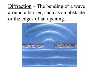
Diffraction
Diffraction. Monday Nov. 18, 2002. Diffraction theory (10.4 Hecht). We will first develop a formalism that will describe the propagation of a wave – that is develop a mathematical description of Huygen’s principle. Wavefront U. What is U here?. We know this. Diffraction theory.

Diffraction
E N D
Presentation Transcript
Diffraction Monday Nov. 18, 2002
Diffraction theory (10.4 Hecht) • We will first develop a formalism that will describe the propagation of a wave – that is develop a mathematical description of Huygen’s principle Wavefront U What is U here? We know this
Diffraction theory • Consider two well behaved functions U1’, U2’ that are solutions of the wave equation. • Let U1’ = U1e-it ; U2’ = U2e-it • Thus U1 , U2 are the spatial part of the functions and since, • we have,
Green’s theorem • Consider the product U1 grad U2 = U1U2 • Using Gauss’ Theorem • Where S = surface enclosing V • Thus,
Green’s Theorem • Now expand left hand side, • Do the same for U2U1 and subtract from (2), gives Green’s theorem
Green’s theorem • Now for functions satisfying the wave equation (1), i.e. • Consequently, • since the LHS of (3) = 0
Green’s theorem applied to spherical wave propagation • Let the disturbance at t=0 be, where r is measured from point P in V and U1 = “Green’s function” • Since there is a singularity at the point P, draw a small sphere P, of radius , around P (with P at centre) • Then integrate over +P, and take limit as 0
Spherical Wave propagation P Thus (4) can be written,
Spherical Wave propagation • In (5), an element of area on P is defined in terms of solid angle • and we have used • Now consider first term on RHS of (5)
Kirchoff’s Integral Theorem • Now U2 = continuous function and thus the derivative is bounded (assume) • Its maximum value in V = C • Then since eik 1 as 0 we have, • The second term on the RHS of (5)
Kirchoff’s Integral Theorem Now as 0 U2(r) UP (its value at P) and, Now designate the disturbance U as an electric field E
Kirchoff integral theorem This gives the value of disturbance at P in terms of values on surface enclosing P. It represents the basic equation of scalar diffraction theory
Geometry of single slit Have infinite screen with aperture A Let the hemisphere (radius R) and screen with aperture comprise the surface () enclosing P. P S r r’ ’ Radiation from source, S, arrives at aperture with amplitude Since R E=0 on . R Also, E = 0 on side of screen facing V.
Fresnel-Kirchoff Formula • Thus E=0 everywhere on surface except the portion that is the aperture. Thus from (6)
Fresnel-Kirchoff Formula • Now assume r, r’ >> ; then k/r >> 1/r2 • Then the second term in (7) drops out and we are left with, Fresnel Kirchoff diffraction formula
Obliquity factor • Since we usually have ’ = - or n.r’=-1, the obliquity factor F() = ½ [1+cos ] • Also in most applications we will also assume that cos 1 ; and F() = 1 • For now however, keep F()
Huygen’s principle • Amplitude at aperture due to source S is, • Now suppose each element of area dA gives rise to a spherical wavelet with amplitude dE = EAdA • Then at P, • Then equation (6) says that the total disturbance at P is just proportional to the sum of all the wavelets weighted by the obliquity factor F() • This is just a mathematical statement of Huygen’s principle.
In Fraunhofer diffraction, both incident and diffracted waves may be considered to be plane (i.e. both S and P are a large distance away) If either S or P are close enough that wavefront curvature is not negligible, then we have Fresnel diffraction Fraunhofer vs. Fresnel diffraction S P Hecht 10.2 Hecht 10.3
Fraunhofer vs. Fresnel Diffraction ’ r’ r h’ h d’ S P d
Fraunhofer Vs. Fresnel Diffraction Now calculate variation in (r+r’) in going from one side of aperture to the other. Call it
Fraunhofer diffraction limit sin’ sin • Now, first term = path difference for plane waves ’ sin’≈ h’/d’ sin ≈ h/d sin’ + sin = ( h’/d + h/d ) Second term = measure of curvature of wavefront Fraunhofer Diffraction
Fraunhofer diffraction limit • If aperture is a square - X • The same relation holds in azimuthal plane and 2 ~ measure of the area of the aperture • Then we have the Fraunhofer diffraction if, Fraunhofer or far field limit
Fraunhofer, Fresnel limits • The near field, or Fresnel, limit is • See 10.1.2 of text
Fraunhofer diffraction • Typical arrangement (or use laser as a source of plane waves) • Plane waves in, plane waves out screen S f1 f2
Fraunhofer diffraction • Obliquity factor Assume S on axis, so Assume small ( < 30o), so • Assume uniform illumination over aperture r’ >> so is constant over the aperture • Dimensions of aperture << r r will not vary much in denominator for calculation of amplitude at any point P consider r = constant in denominator
Fraunhofer diffraction • Then the magnitude of the electric field at P is,
Single slit Fraunhofer diffraction P y = b r dy ro y r = ro - ysin dA = L dy where L ( very long slit)
Single slit Fraunhofer diffraction Fraunhofer single slit diffraction pattern