Download
1 / 30
320 likes | 541 Views
Introduction to Statistics: Political Science (Class 2). Central Limit Theorem, T-statistics, and using split sample analysis and multivariate regression to deal with confounds. Today…. A review of what standard errors and T-statistics tell us Multivariate regression.

E N D
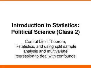
Introduction to Statistics: Political Science (Class 2) Central Limit Theorem, T-statistics, and using split sample analysis and multivariate regression to deal with confounds
Today… • A review of what standard errors and T-statistics tell us • Multivariate regression
The goal of statistical analysis? • We want to know: *true* “population” mean or relationship • What we have: sample of the units we are interested in • Thus we estimate the mean or relationship • What is an estimate?
Actually we estimate 2 things • Estimate of mean or relationship • We know how to get this (calculate the mean or find the best fit line) • Estimate of uncertainty • Often (typically?): How confident can we be that a mean or relationship is not zero • We can’t measure our uncertainty directly (we’re uncertain – duh!)
The Central Limit Theorem • In repeated sampling (if we redrew over and over and over and recalculated)… • the average of the estimates will be centered on the population (“true”) mean • the distribution of estimates will be approximately normal…
Like this • This width depends on: • Variance in population (more wider) • Number of cases sampled (more narrower)
Mean ideology of the American public • How would you rate yourself on the following scale? • Very Liberal • Liberal • Somewhat Liberal • Middle of the Road • Somewhat Conservative • Conservative • Very Conservative • If we were omniscient (or could ask every single person) we would know that the true average is 5.0 • but we’re not/we can’t…Instead we call 100 people at random… and then we do that again and again…
In any given sample we would be about 95% confident that the true population mean was somewhere within this range Estimating Mean Ideology
One Standard Error Another way to think about this is that 95% of the time, our estimates of the mean will be within about +/- two standard errors of the population value 5.0
So T can be thought of as: how many SEs from 0 that the coefficient is Coef SE Coef T P Democracy Scores 0.259 0.023 11.34 0.000 Constant 23.21 0.253 91.82 0.000 Same idea with regression coefficient • If we were able to redraw new samples over and over and re-estimate β… • Typically (always for our purposes here) we’re testing whether a coefficient = 0
0 T = -11.34 T = 11.34 If the true relationship was 0 (no relationship), getting an estimated coefficient with a T-value with an absolute value greater than 11.34 by chance would be extremely unlikely(about 1 in 1,000,000,000,000,000,000,000,000,000,000) So we can be confident rejecting the null hypotheses (What’s the null? Why do we set things up this way?)
1 v. 2-tailed tests 1-tailed: You have strong prior expectations about direction of relationship (if relationship turns out to be in the other direction you can’t reject the null – even w/a large t-statistic) 2-tailed: No strong priors about direction of relationship – more conservative test
Causal relationships • Identifying associations is nice, but usually we want to identify causality • Two primary threats • Reverse causation (we’ll table this for now and talk about it in a few weeks) • Confounding variablesNeed to rule out alternative explanations
Bush was particularly unpopular at the end of his presidency… How much did bad feelings about Bush help Obama? ? Feelings about Bush Feelings about Obama
Measuring “reverse coattails” effect …I'll read the name of a person and I'd like you to rate that person using something we call the feeling thermometer. Ratings between 50 degrees and 100 degrees mean that you feel favorable and warm toward the person. Ratings between 0 degrees and 50 degrees mean that you don't feel favorable toward the person and that you don't care too much for that person. You would rate the person at the 50 degree mark if you don't feel particularly warm or cold toward the person. Bivariate regression Υ = β0 + β1X + u SO… Obama FT = β0 + β1(Bush FT) + u
Obama FT = 80.4 + (-0.43*Bush FT) Coef. SE T P-value Bush FT -.43 .018 -24.12 0.000 Constant 80.4 .852 94.37 0.000 R-squared = 0.203
What else might explain this (strong!) relationship? • Other factors that might affect evaluations of both Obama and Bush?
Party Identification? Party Identification Bush Feeling Thermometer Obama Feeling Thermometer
Party Identification • Generally speaking, do you usually think of yourself as a Democrat, a Republican, an Independent, or what? -3 = Strong Republican -2 = Weak Republican -1 = Lean Republican 0 = Independent 1 = Lean Democrat 2 = Weak Democrat 3 = Strong Democrat
Party Identification FTs Predict Obama Feeling Thermometer Coef. SE T P-value Party Identification 8.71 .234 37.16 0.000 Constant 58.1 .507 114.71 0.000 Predict Bush Feeling Thermometer Coef. SE T P-value Party Identification -8.19 .259 -31.58 0.000 Constant 43.3 .560 77.38 0.000
Accounting for a confound by splitting the sample… • Among Democrats: • Mean evaluation of Bush: 24.7 • Mean evaluation of Obama: 79.2 • Among Republicans: • Mean evaluation of Bush: 65.9 • Mean evaluation of Obama: 35.5 • Let’s see what happens when we run separate regressions for Democrats and Republicans…
Model with all respondents Obama FT = 80.4 + (-0.43*Bush FT)
We only want to give Bush FT explanatory “credit” for this part of the relationship Not this part Party ID as Confound Bush Feeling Thermometer (X) Obama Feeling Thermometer (Y) Party Identification (Z)
Multivariate Regression Υ = β0 + β1X + β2X + u Obama FT = β0 + β1(Bush FT) + β2(Party Identification) + u (party identification -3=strong Republican; 3=strong Democrat)
Multivariate Regression Language: relationship between X1 and Y controlling for X2 (OR holding X2 constant) (more precisely: “controlling for the linear relationship between X2 and Y”) Coef. St.Err T P Bush FT -.165 .019 -8.72 0.000 Party Identification 7.354 .278 26.44 0.000 Constant 65.28 .962 67.89 0.000
Bush FT only gets “credit” for this part of the overlap Bivariate regression: Bush FT gets “credit” for all of this overlap Party Affiliation No variable gets “credit” for this part, (but it does affect the R-squared) Party Affiliation only gets “credit” for this part of the overlap Bush Feeling Thermometer Obama Feeling Thermometer
Getting predicted values Obama FT = β0 + β1(Bush FT) + β2 (Party Identification) + u Coef. St.Err T P Bush FT -.165 .019 -8.72 0.000 Party Identification 7.354 .278 26.44 0.000 Constant 65.28 .962 67.89 0.000
Getting predicted values Obama FT = 65.28 + (-.165)(Bush FT) + 7.354(Party Identification) + u What does the coefficient on the constant mean? Expected Value for a Strong Democrat who gave Bush a feeling thermometer rating of 50? Coef. St.Err T P Bush FT -.165 .019 -8.72 0.000 Party Identification 7.354 .278 26.44 0.000 Constant 65.28 .962 67.89 0.000
Notes and Next Time • No Class on Tuesday • Remember to look at the homework assignment in time to get TA office hour help before it’s due next Thursday! • Next time: • R-squared • Non-continuous explanatory variables • Joint significance of variables (F-tests)