Download

1 / 26
260 likes | 408 Views
Labor, Employment And Wages. Samuel Bowles Santa Fe Institute University of Siena. Diego Rivera, The Ford Plant River Rouge. Employment: what is the principal agent problem?. e 0 [0,1] = effort per hour of work (e.g. % of time “on”) Per period output is:

E N D
Labor, Employment And Wages Samuel Bowles Santa Fe Institute University of Siena Diego Rivera, The Ford Plant River Rouge
Employment: what is the principal agent problem? • e 0 [0,1] = effort per hour of work (e.g. % of time “on”) • Per period output is: y = y(he) + µ , with y'>0 and y" <0; where h is the number of worker "hours" hired µ is a mean zero disturbance term. • the employer selects i) termination probability t(e,m)0[0,1] (te<0 and tm>0 ii) a wage rate, w, and iii) monitoring expenditure per hour of labor hired, m • the worker selects e to max his present value of utility • the worker is paid, and is renewed or terminated, the latter occurring with probability t(e,m).
The Worker’s Best Response • Per period utility (experienced at the end of the period) u = u(w,e) • Fallback asset Z: what is it? • Present value of the job (game is stationary): V = {u(w,e)+(1-t(e,m))V+t(e,m)Z}'(1+i) V = {u(w,e)-iZ}'(i+t(e,m) + Z • The worker selects e so as to set Ve = 0 • which requires: ue = te(V-Z) • Interpretation of the foc? • Given that P knows A’s brf, he also knows the resulting e. Why then is there a P-A problem?
The Worker’s Fallback Position • At the end of each period there is a probability λ that the unemployed worker will find work, exiting the unemployment pool, so the expected duration of unemployment is 1/λ. • Thus Z = {u(b,0)+λV+(1-λ)Z}'(1+i) = {u(b,0)+λV'(i +λ)
Employee’s best response function: ue = te(V-Z) • slope of iso-v? • {e , w}?
Profit Maximizing • π = y(he(w,m;Z)) - (w+m)h • πh = y'e - (w+m) = 0 • πw = y'hew - h = 0 • πm = y'hem - h = 0 • which requires that ew = e/(w+m) = em y'= (w+m)/e • Meaning of the second foc?
The Solow condition: ew = e/(w+m) = em • What does it mean? • Show that a Walrasian equilibrium is a special case of this model. • What does it require of the nature of work and the scarcity of goods?
Comparative Statics • Let (w+m)/e / μ the cost of a unit effort • dμ/dZ > 0; and dπ/dZ < 0 • What is the economic meaning of these results?
General Equilibrium • The zero profit condition π - δ = 0 • λ varies with the level of aggregate employment (nh=H), so • λ = λ(H, ...) with λ’> 0 • Z = Z(H, ..) with Z’ > 0 • Recall that (w+m)/e / μ the cost of a unit effort and dμ/dZ > 0 and dπ/dZ < 0 • Because these relationships are all monotonic, there is a unique μ0 and hence a unique Z0 and H0 that satisfies the zpc. • Thus the level of unemployment, employment, number of firms are determined. Why is H<1? • No reference to aggregate demand?
e*, w*is Pareto-inefficient. Why? How to show this? • Ve = 0 but πe > 0 and Vw > 0 but πw = 0; • thus there exists some (arbitrarily small) values (Δe,Δw) such that V(e*+Δe,w*+Δw)>V(e*,w*) and π(e*+Δe,w*+Δw,...)>π(e*,w*) € • Where is the efficient contract locus in the figure?
Why is w*, m* technically inefficient? In what sense is m unproductive labor?
Pareto sub-optimal workplace amenities • Suppose the employee's utility function is expanded to include a measure of work amenities provided (per hour of work), τ u=(w,τ,e) with uτ > 0 over the relevant range, and that amenities cost pτ for the employer to provide. • a new present value V(e,w,τ) • a new best response function e(w,m,τ;z) • an additional first order condition for the employer πτ = y'eτ - pτ = 0 • Q: Why will τ* be P-suboptimal? • A: for the same reason that the wage suboptimal: more amenities and more effort are a pareto improvement
Can trade union bargaining implement a P-improvement over w*,e*? The Employer’s and Union’s Bargaining Problem: Per Period Payoffs (right figure) Note the bargaining set is the area bounded by the payoffs in the non cooperative interaction and the efficient contract locus. If the strategies available were unconditional w+ and w* for the employer and e+ and e* for the employee, the game is a prisoners dilemma. Point a is the equilibrium of the uncooperative game (indicated by point a in the left figure) while point b is a point on the efficient contract locus (indicated by point b in figure 1).
Given that job rents are huge, firms could sell jobs. What problem would the firm solve to calculate the optimal fee? • Let B = a one time job fee. • The employer varies h, w, and B to maximize π = y(he(w)) -hw + iBh subject to V(e(w), w-iB) $ Z where i is the rate of return and V(.) is the ex ante present value of the job with fee B. • w-iB is the net wage taking account of the opportunity cost to the employee of foregoing returns iB on the employee’s wealth.
Results: • P-efficient? • Labor market clearing? • P has power over A? Optimal job fees. The employer identifies point a as the solution of max e/(m+w-iB), the effort elicited from the employee per unit cost. The employer then offers w* (the employee responds with e*) with a fee of B*.
Why do firms not sell jobs (charge an optimal fee)? Some possible answers • Firm’s search costs are reduced by job rationing • Morale, reciprocity reasons • Perhaps they do (by very low initial wages, etc)
Macroeconomic applications • w*(h): the labor market equilibrium (workers and firms foc with respect to labor discipline); h is total employment • h*(w): the locus of {w,h} s.t. excess demand for goods = i + b – s = 0 • Upward shift in w*(h) increases h*; saving depends strongly on profit share Bowles, Samuel and Robert Boyer. 1988. "Labor Discipline and Aggregate Demand: A Macroeconomic Model." American Economic Review, 78:2, pp. 395-400.
Two ways of closing the model: zpc or aggregate demand • h* (w) could be the h for a given w that satisfies zpc (necessarily downwards sloping) or • …the level of employment that clears the product market.
Evidence • Labor effort appears to be quite variable and is rarely subject to contract (Laffont, Lazear, Rosenzweig et al) • Employers devote substantial personnel (Gordon) and other resources (Baker) to monitoring their employees’ effort. • Substantial employment rents in most jobs ( primary /secondary labor market distinction) (Weisskopf and Green) • Real wages tend to vary with the level of employment (Blanchflower and Oswald, Bowles, BER) • Econometric evidence on effort (Schor), labor productivity (BGW), and profits (BGW) (high employment profit squeeze) • Experimental evidence (Fehr et al) • Footnote: how BGW came to do this work.
Presentations of discussion questions (with .ppt or handouts) • Apartheid as labor discipline (22.3) • The distribution of gains from freer North South trade (22.2) • An employment subsidy with endogenous effort (23) • An incentive compatible BIG (unconditional basic income grant) (24) • Husbands and wives/Principals and agents (29) A more extensive review of the evidence, if you’d like Next : credit and wealth, read chapter 9.
Additional readings • Bowles, Samuel, Herbert Gintis, and Melissa Osborne. 2001. "Incentive-Enhancing Preferences." American Economic Review, 91:2, pp. 155-58 • Heckman, James and Yona Rubinstein. 2001. "The importance of non-cognitive skills: lessons from the GED testing progam." American Economic Review, 91:2, pp. 145-49 • Bowles, Samuel, Herbert Gintis, and Melissa Osborne. 2001. "The Determinants of Earnings: A Behavioral Approach." Journal of Economic Literature, XXXIX(December), pp. 1137-76.
After NAFTA. A country (South) with a large traditional grain growing sector protected by tariffs and subsidies shares a border with a country (North) with ideal grain growing conditions and a highly productive agricultural sector. The reservation position for wage workers in the South is to return to working on their family's farm in the traditional agricultural sector. An international trade economist proposes a free trade area for the two countries, removing tariffs and subsidies, showing that substantial gains from trade will result for both countries, and claiming that employees in the South will enjoy higher (real) wages as a result. A worker asks you if the claim is correct. The trade economist is certainly right about the gains from trade; but what about the wage increases? Show that i) using the no shirking condition as the model of wage determination, the trade economist is wrong and ii) assuming that wages and effort are determined by a Nash bargain between employees and employers he could be right, but need not be.
The apartheid system in South Africa gave non-white workers restricted access to the labor market of the modern sector of the economy. According to the infamous pass laws, those working in the urban areas required a pass, which was revoked if their job was terminated, and they were required to return to close to subsistence living in one of the so- called bantustans. South African scholars have debated whether this system lowered profits (by restricting the supply of labor) or raised profits (by providing businesses with a favorable labor discipline environment). Use the labor discipline model (the no shirking condition, or the more general model in the text) to develop the latter argument. What additional information would you need to determine which position is more nearly correct?
A wage subsidy. Employment subsidies are a widely discussed means of increasing employment in labor surplus economies, or among less skilled workers in the advanced countries. Suppose that n identical firms each hire h hours of identical labor, varying both h and w, the hourly wage, to maximize profits, which depend on total labor effor which is the product of hours hired and effort per hour, e. Consider two types of subsidy paid to owners of each firm: i) an employment subsidy: the subsidy s is a fixed amount, paid per hour of labor hired, or ii) a wage subsidy, F, the subsidy is a fixed fraction of the wages paid. You may assume that the taxes supporting this subsidy have no effects on this problem. Using the zero subsidy case as a benchmark, indicate the effects of the two types of subsidy on the equilibrium wage, effort, and employment levels, assuming a) that z,the fallback position of each worker, is exogenous, and b) that z varies with the level of total employment, nh
The BIG idea. (§8) Assume all employed work for an hour. A linear tax (meaning with a flat rate, J) is levied on every employed worker, the proceeds being distributed unconditionally to all members of the population (for simplicity, assume that half of those in the population are employed, a quarter are unemployed and a quarter are not in the labor force). Because profits are not taxed and because all workers (including those not working) are identical, we assume this proposal has no effect on the demand for labor so the expected duration of a spell of unemployment is unaffected. You may also abstract from any changes in labor supply. Assume that the implementation of the BIG is accompanied by the elimination of unemployment insurance (define this as b), the replacement income a worker receives if unemployed) and that the net effect of the tax, the BIG, and the elimination of unemployment insurance on the government budget is zero. If the employment relationship is governed by the contingent renewal model in the text, with w=w*, e=e* with b = w*/2 what is the maximum tax that can be levied without reducing the equilibrium level of effort and what is the resulting per person grant? Check to see that a family composed of two employed workers, one unemployed person and one out of the labor force, experiences no change in income or total effort provided, while those with relatively more non-employed members gain.
Domestic labor. (§10) Consider the determination of domestic work and the sharing of income by a husband and wife (the amount of domestic work done is not costlessly observable by the other adult, as much of it is bestowed on the children, and the results of this are only evident in the very long run). Consider only the two adults, one of whom works for pay and other works in their home. Extend the model in chapter 8 to determine the share of the paid worker's income received by the home worker (w) and the amount of domestic work done (e). Contrast this “domestic labor discipline” model with a transactions cost approach to this problem. What are the relevant transaction specific investments? What are the similarities and key differences?