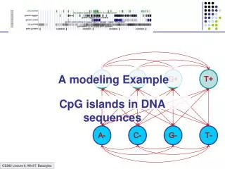
A modeling Example
This article explores the significance of CpG islands in DNA sequences, focusing on the role of methylation in gene silencing and cellular differentiation. Methylation, indicated by the addition of a CH₃ group to cytosines, often silences nearby genes and plays a critical role in the inheritance of traits during cell division. We discuss computational methods for detecting CpG islands and propose a model that incorporates transitions and emission probabilities to differentiate between CpG and non-CpG islands. The article also addresses parameter estimation in novel genomes like the porcupine and methods to mitigate overfitting in data.
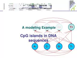

A modeling Example
E N D
Presentation Transcript
A+ C+ G+ T+ A- C- G- T- A modeling Example CpG islands in DNA sequences
Methylation & Silencing • One way cells differentiate is methylation • Addition of CH3 in C-nucleotides • Silences genes in region • CG (denoted CpG) often mutates to TG, when methylated • In each cell, one copy of X is silenced, methylation plays role • Methylation is inherited during cell division
Example: CpG Islands CpG nucleotides in the genome are frequently methylated (Write CpG not to confuse with CG base pair) C methyl-C T Methylation often suppressed around genes, promoters CpG islands
Example: CpG Islands • In CpG islands, • CG is more frequent • Other pairs (AA, AG, AT…) have different frequencies Question: Detect CpG islands computationally
A model of CpG Islands – (1) Architecture A+ C+ G+ T+ CpG Island A- C- G- T- Not CpG Island
A model of CpG Islands – (2) Transitions How do we estimate parameters of the model? Emission probabilities: 1/0 • Transition probabilities within CpG islands Established from known CpG islands (Training Set) • Transition probabilities within other regions Established from known non-CpG islands (Training Set) Note: these transitions out of each state add up to one—no room for transitions between (+) and (-) states = 1 = 1 = 1 = 1 = 1 = 1 = 1 = 1
Log Likehoods—Telling “CpG Island” from “Non-CpG Island” Another way to see effects of transitions: Log likelihoods L(u, v) = log[ P(uv | + ) / P(uv | -) ] Given a region x = x1…xN A quick-&-dirty way to decide whether entire x is CpG P(x is CpG) > P(x is not CpG) i L(xi, xi+1) > 0
A model of CpG Islands – (2) Transitions • What about transitions between (+) and (-) states? • They affect • Avg. length of CpG island • Avg. separation between two CpG islands 1-p Length distribution of region X: P[lX = 1] = 1-p P[lX = 2] = p(1-p) … P[lX= k] = pk-1(1-p) E[lX] = 1/(1-p) Geometric distribution, with mean 1/(1-p) X Y p q 1-q
What if a new genome comes? • We just sequenced the porcupine genome • We know CpG islands play the same role in this genome • However, we have no known CpG islands for porcupines • We suspect the frequency and characteristics of CpG islands are quite different in porcupines How do we adjust the parameters in our model? LEARNING
Learning Re-estimate the parameters of the model based on training data
Two learning scenarios • Estimation when the “right answer” is known Examples: GIVEN: a genomic region x = x1…x1,000,000 where we have good (experimental) annotations of the CpG islands GIVEN: the casino player allows us to observe him one evening, as he changes dice and produces 10,000 rolls • Estimation when the “right answer” is unknown Examples: GIVEN: the porcupine genome; we don’t know how frequent are the CpG islands there, neither do we know their composition GIVEN: 10,000 rolls of the casino player, but we don’t see when he changes dice QUESTION: Update the parameters of the model to maximize P(x|)
1. When the right answer is known Given x = x1…xN for which the true = 1…N is known, Define: Akl = # times kl transition occurs in Ek(b) = # times state k in emits b in x We can show that the maximum likelihood parameters (maximize P(x|)) are: Akl Ek(b) akl = ––––– ek(b) = ––––––– i AkicEk(c)
1. When the right answer is known Intuition: When we know the underlying states, Best estimate is the normalized frequency of transitions & emissions that occur in the training data Drawback: Given little data, there may be overfitting: P(x|) is maximized, but is unreasonable 0 probabilities – BAD Example: Given 10 casino rolls, we observe x = 2, 1, 5, 6, 1, 2, 3, 6, 2, 3 = F, F, F, F, F, F, F, F, F, F Then: aFF = 1; aFL = 0 eF(1) = eF(3) = .2; eF(2) = .3; eF(4) = 0; eF(5) = eF(6) = .1
Pseudocounts Solution for small training sets: Add pseudocounts Akl = # times kl transition occurs in + rkl Ek(b) = # times state k in emits b in x + rk(b) rkl, rk(b) are pseudocounts representing our prior belief Larger pseudocounts Strong priof belief Small pseudocounts ( < 1): just to avoid 0 probabilities
Pseudocounts Example: dishonest casino We will observe player for one day, 600 rolls Reasonable pseudocounts: r0F = r0L = rF0 = rL0 = 1; rFL = rLF = rFF = rLL = 1; rF(1) = rF(2) = … = rF(6) = 20 (strong belief fair is fair) rL(1) = rL(2) = … = rL(6) = 5 (wait and see for loaded) Above #s are arbitrary – assigning priors is an art
2. When the right answer is unknown We don’t know the true Akl, Ek(b) Idea: • We estimate our “best guess” on what Akl, Ek(b) are • Or, we start with random / uniform values • We update the parameters of the model, based on our guess • We repeat
2. When the right answer is unknown Starting with our best guess of a model M, parameters : Given x = x1…xN for which the true = 1…N is unknown, We can get to a provably more likely parameter set i.e., that increases the probability P(x | ) Principle: EXPECTATION MAXIMIZATION • Estimate Akl, Ek(b) in the training data • Update according to Akl, Ek(b) • Repeat 1 & 2, until convergence
Estimating new parameters To estimate Akl: (assume “|CURRENT”, in all formulas below) At each position i of sequence x, find probability transition kl is used: P(i = k, i+1 = l | x) = [1/P(x)] P(i = k, i+1 = l, x1…xN) = Q/P(x) where Q = P(x1…xi, i = k, i+1 = l, xi+1…xN) = = P(i+1 = l, xi+1…xN | i = k) P(x1…xi, i = k) = = P(i+1 = l, xi+1xi+2…xN | i = k) fk(i) = = P(xi+2…xN | i+1 = l) P(xi+1 | i+1 = l) P(i+1 = l | i = k) fk(i) = = bl(i+1) el(xi+1) akl fk(i) fk(i) akl el(xi+1) bl(i+1) So: P(i = k, i+1 = l | x, ) = –––––––––––––––––– P(x | CURRENT)
Estimating new parameters • So, Akl is the E[# times transition kl, given current ] fk(i) akl el(xi+1) bl(i+1) Akl = i P(i = k, i+1 = l | x, ) = i ––––––––––––––––– P(x | ) • Similarly, Ek(b) = [1/P(x | )]{i | xi = b} fk(i) bk(i) fk(i) bl(i+1) akl k l xi+2………xN x1………xi-1 el(xi+1) xi xi+1
The Baum-Welch Algorithm Initialization: Pick the best-guess for model parameters (or arbitrary) Iteration: • Forward • Backward • Calculate Akl, Ek(b), given CURRENT • Calculate new model parameters NEW : akl, ek(b) • Calculate new log-likelihood P(x | NEW) GUARANTEED TO BE HIGHER BY EXPECTATION-MAXIMIZATION Until P(x | ) does not change much
The Baum-Welch Algorithm Time Complexity: # iterations O(K2N) • Guaranteed to increase the log likelihood P(x | ) • Not guaranteed to find globally best parameters Converges to local optimum, depending on initial conditions • Too many parameters / too large model: Overtraining
Alternative: Viterbi Training Initialization: Same Iteration: • Perform Viterbi, to find * • Calculate Akl, Ek(b) according to * + pseudocounts • Calculate the new parameters akl, ek(b) Until convergence Notes: • Not guaranteed to increase P(x | ) • Guaranteed to increase P(x | , *) • In general, worse performance than Baum-Welch