Download
1 / 21
210 likes | 808 Views
Measures of Dispersion & The Standard Normal Distribution. 2/5/07. The Semi-Interquartile Range (SIR). A measure of dispersion obtained by finding the difference between the 75 th and 25 th percentiles and dividing by 2. Shortcomings

E N D
Measures of Dispersion&The Standard Normal Distribution 2/5/07
The Semi-Interquartile Range (SIR) • A measure of dispersion obtained by finding the difference between the 75th and 25th percentiles and dividing by 2. • Shortcomings • Does not allow for precise interpretation of a score within a distribution • Not used for inferential statistics.
Calculate the SIR 6, 7, 8, 9, 9, 9, 10, 11, 12 • Remember the steps for finding quartiles • First, order the scores from least to greatest. • Second, Add 1 to the sample size. • Third, Multiply sample size by percentile to find location. • Q1 = (10 + 1) * .25 • Q2 = (10 + 1) * .50 • Q3 = (10 + 1) * .75 • If the value obtained is a fraction take the average of the two adjacent X values.
Variance (second moment about the mean) • The Variance, s2, represents the amount of variability of the data relative to their mean • As shown below, the variance is the “average” of the squared deviations of the observations about their mean • The Variance, s2, is the sample variance, and is used to estimate the actual population variance, s 2
Standard Deviation • Considered the most useful index of variability. • Can be interpreted in terms of the original metric • It is a single number that represents the spread of a distribution. • If a distribution is normal, then the mean plus or minus 3 SD will encompass about 99% of all scores in the distribution.
Definitional vs. Computational • Definitional • An equation that defines a measure • Computational • An equation that simplifies the calculation of the measure
Interpreting the standard deviation • We can compare the standard deviations of different samples to determine which has the greatest dispersion. • Example • A spelling test given to third-grader children 10, 12, 12, 12, 13, 13, 14 xbar = 12.28 s = 1.25 • The same test given to second- through fourth-grade children. 2, 8, 9, 11, 15, 17, 20 xbar = 11.71 s = 6.10
Interpreting the standard deviation • Remember • Fifty Percent of All Scores in a Normal Curve Fall on Each Side of the Mean
The shape of distributions • Skew • A statistic that describes the degree of skew for a distribution. • 0 = no skew • + or - .50 is sufficiently symmetrical • + value = + skew • - value = - skew • You are not expected to calculate by hand. • Be able to interpret
Kurtosis • Mesokurtic (normal) • Around 3.00 • Platykurtic (flat) • Less than 3.00 • Leptokurtic (peaked) • Greater than 3.00 • You are not expected to calculate by hand. • Be able to interpret
The Standard Normal Distribution • Z-scores • A descriptive statistic that represents the distance between an observed score and the mean relative to the standard deviation
Standard Normal Distribution • Z-scores • Convert a distribution to: • Have a mean = 0 • Have standard deviation = 1 • However, if the parent distribution is not normal the calculated z-scores will not be normally distributed.
Why do we calculate z-scores? • To compare two different measures • e.g., Math score to reading score, weight to height. • Area under the curve • Can be used to calculate what proportion of scores are between different scores or to calculate what proportion of scores are greater than or less than a particular score. • Used to set cut score for screening instruments.
Class practice 6, 7, 8, 9, 9, 9, 10, 11, 12 Calculate z-scores for 8, 10, & 11. What percentage of scores are greater than 10? What percentage are less than 8? What percentage are between 8 and 10?
Z-scores to raw scores • If we want to know what the raw score of a score at a specific %tile is we calculate the raw using this formula. • With previous scores what is the raw score • 90%tile • 60%tile • 15%tile
Transformation scores • We can transform scores to have a mean and standard deviation of our choice. • Why might we want to do this?
With our scores • We want: • Mean = 100 • s = 15 • Transform: • 8 & 10.
Key points about Standard Scores • Standard scores use a common scale to indicate how an individual compares to other individuals in a group. • The simplest form of a standard score is a Z score. • A Z score expresses how far a raw score is from the mean in standard deviation units. • Standard scores provide a better basis for comparing performance on different measures than do raw scores. • A Probability is a percent stated in decimal form and refers to the likelihood of an event occurring. • T scores are z scores expressed in a different form (z score x 10 + 50).