Download
1 / 43
450 likes | 705 Views
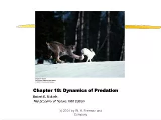
Chapter 18: Dynamics of Predation. Robert E. Ricklefs The Economy of Nature, Fifth Edition. Population Cycles of Canadian Hare and Lynx. Charles Elton’s seminal paper focused on fluctuations of mammals in the Canadian boreal forests.

E N D
Chapter 18: Dynamics of Predation Robert E. Ricklefs The Economy of Nature, Fifth Edition (c) 2001 by W. H. Freeman and Company
Population Cycles of Canadian Hare and Lynx • Charles Elton’s seminal paper focused on fluctuations of mammals in the Canadian boreal forests. • Elton’s analyses were based on trapping records maintained by the Hudson’s Bay Company • of special interest in these records are the regular and closely linked fluctuations in populations of the lynx and its principal prey, the snowshoe hare • What causes these cycles? (c) 2001 by W. H. Freeman and Company
Some Fundamental Questions • The basic question of population biology is: • what factors influence the size and stability of populations? • Because most species are both consumers and resources for other consumers, this basic question may be refocused: • are populations limited primarily by what they eat or by what eats them? (c) 2001 by W. H. Freeman and Company
More Questions • Do predators reduce the size of prey populations substantially below the carrying capacity set by resources for the prey? • this question is prompted by interests in management of crop pests, game populations, and endangered species • Do the dynamics of predator-prey interactions cause populations to oscillate? • this question is prompted by observations of predator-prey cycles in nature, such as Elton’s lynx and hare (c) 2001 by W. H. Freeman and Company
Consumers can limit resource populations. • An example: populations of cyclamen mites, a pest of strawberry crops in California, can be regulated by a predatory mite: • cyclamen mites typically invade strawberry crops soon after planting and build to damaging levels in the second year • predatory mites invade these fields in the second year and keep cyclamen mites in check • Experimental plots in which predatory mites were controlled by pesticide had cyclamen mite populations 25 times larger than untreated plots. (c) 2001 by W. H. Freeman and Company
What makes an effective predator? • Predatory mites control populations of cyclamen mites in strawberry plantings because, like other effective predators: • they have a high reproductive capacity relative to that of their prey • they have excellent dispersal powers • they can switch to alternate food resources when their primary prey are unavailable (c) 2001 by W. H. Freeman and Company
Consumer Control in Aquatic Ecosystems • An example: sea urchins exert strong control on populations of algae in rocky shore communities: • in urchin removal experiments, the biomass of algae quickly increases: • in the absence of predation, the composition of the algal community also shifts: • large brown algae replace coralline and small green algae that can persist in the presence of predation (c) 2001 by W. H. Freeman and Company
Predator and prey populations often cycle. • Population cycles observed in Canada are present in many species: • large herbivores (snowshoe hares, muskrat, ruffed grouse, ptarmigan) have cycles of 9-10 years: • predators of these species (red foxes, lynx, marten, mink, goshawks, owls) have similar cycles • small herbivores (voles and lemmings) have cycles of 4 years: • predators of these species (arctic foxes, rough-legged hawks, snowy owls) also have similar cycles • cycles are longer in forest, shorter in tundra (c) 2001 by W. H. Freeman and Company
Predator-Prey Cycles: A Simple Explanation • Population cycles of predators lag slightly behind population cycles of their prey: • predators eat prey and reduce their numbers • predators go hungry and their numbers drop • with fewer predators, the remaining prey survive better and prey numbers build • with increasing numbers of prey, the predator populations also build, completing the cycle (c) 2001 by W. H. Freeman and Company
Time Lags in Predator-Prey Systems • Delays in responses of births and deaths to an environmental change produce population cycles: • predator-prey interactions have time lags associated with the time required to produce offspring • 4-year and 9- or 10-year cycles in Canadian tundra or forests suggest that time lags should be 1 or 2 years, respectively: • these could be typical lengths of time between birth and sexual maturity • the influence of conditions in one year might not be felt until young born in that year are old enough to reproduce (c) 2001 by W. H. Freeman and Company
Time Lags in Pathogen-Host Systems • Immune responses can create cycles of infection in certain diseases: • measles produced epidemics with a 2-year cycle in pre-vaccine human populations: • two years were required for a sufficiently large population of newly susceptible infants to accumulate (c) 2001 by W. H. Freeman and Company
Time Lags in Pathogen-Host Systems • other pathogens cycle because they kill sufficient hosts to reduce host density below the level where the pathogens can spread in the population: • such cycling is evident in polyhedrosis virus in tent caterpillars • In many regions, tent caterpillar infestations last about 2 years before the virus brings its host population under control • In other regions, infestations may last up to 9 years • Forest fragmentation – which creates abundant forest edge – tends to prolong outbreaks of the tent caterpillar • Why? • Increased forest edge exposes caterpillars to more intense sunlight inactivates the virus thus, habitat manipulation here has secondary effects (c) 2001 by W. H. Freeman and Company
Laboratory Investigations of Predators and Prey • G.F. Gause conducted simple test-tube experiments with Paramecium (prey) and Didinium (predator): • in plain test tubes containing nutritive medium, the predator devoured all prey, then went extinct itself • in tubes with a glass wool refuge, some prey escaped predation, and the prey population reexpanded after the predator went extinct • Gause could maintain predator-prey cycles in such tubes by periodically adding more predators (c) 2001 by W. H. Freeman and Company
Predator-prey interactions can be modeled by simple equations. • Lotka and Volterra independently developed models of predator-prey interactions in the 1920s: dR/dt = rR - cRP describes the rate of increase of the prey population, where: R is the number of prey P is the number of predators r is the prey’s per capita exponential growth rate c is a constant expressing efficiency of predation (c) 2001 by W. H. Freeman and Company
Lotka-Volterra Predator-Prey Equations • A second equation: dP/dt = acRP - dP describes the rate of increase of the predator population, where: P is the number of predators R is the number of prey a is the efficiency of conversion of food to growth c is a constant expressing efficiency of predation d is a constant related to the death rate of predators (c) 2001 by W. H. Freeman and Company
Predictions of Lotka-Volterra Models • Predators and prey both have equilibrium conditions (equilibrium isoclines or zero growth isoclines): • P = r/c for the predator • R = d/ac for the prey • when these values are graphed, there is a single joint equilibrium point where population sizes of predator and prey are stable: • when populations stray from joint equilibrium, they cycle with period T = 2 /rd (c) 2001 by W. H. Freeman and Company
Cycling in Lotka-Volterra Equations • A graph with axes representing sizes of the predator and prey populations illustrates the cyclic predictions of Lotka-Volterra predator-prey equations: • a population trajectory describes the joint cyclic changes of P and R counterclockwise through the P versus R graph (c) 2001 by W. H. Freeman and Company
Factors Changing Equilibrium Isoclines • The prey isocline increases if: • r increases or c decreases, or both: • the prey population would be able to support the burden of a larger predator population • The predator isocline increases if: • d increases and either a or c decreases: • more prey would be required to support the predator population (c) 2001 by W. H. Freeman and Company
Other Lotka-Volterra Predictions • Increasing the predation efficiency (c) alone in the model reduces isoclines for predators and prey: • fewer prey would be needed to sustain a given capture rate • the prey population would be less able to support the more efficient predator • Increasing the birth rate of the prey (r) should lead to an increase in the population of predators but not the prey themselves. (c) 2001 by W. H. Freeman and Company
Modification of Lotka-Volterra Models for Predators and Prey • There are various concerns with the Lotka-Volterra equations: • the lack of any forces tending to restore the populations to the joint equilibrium: • this condition is referred to as a neutral equilibrium • the lack of any satiation of predators: • each predator consumes a constant proportion of the prey population regardless of its density (c) 2001 by W. H. Freeman and Company
The Functional Response • A more realistic description of predator behavior incorporates alternative functional responses, proposed by C.S. Holling: • type I response: rate of consumption per predator is proportional to prey density (no satiation) • type II response: number of prey consumed per predator increases rapidly, then plateaus with increasing prey density • type III response: like type II, except predator response to prey is depressed at low prey density (c) 2001 by W. H. Freeman and Company
The Holling Type III Response • What would cause the type III functional response? • heterogeneous habitat, which provides a limited number of safe hiding places for prey • lack of reinforcement of learned searching behavior due to a low rate of prey encounter • switching by predator to alternative food sources when prey density is low (c) 2001 by W. H. Freeman and Company
The Numerical Response • If individual predators exhibit satiation (type II or III functional responses), continued predator response to prey must come from: • increase in predator population through local population growth or immigration from elsewhere • this increase is referred to as a numerical response (c) 2001 by W. H. Freeman and Company
Several factors reduce predator-prey oscillations. • All of the following tend to stabilize predator and prey numbers (in the sense of maintaining nonvarying equilibrium population sizes): • predator inefficiency • density-dependent limitation of either predator or prey by external factors • alternative food sources for the predator • refuges from predation at low prey densities • reduced time delays in predator responses to changes in prey abundance (c) 2001 by W. H. Freeman and Company
Destabilizing Influences • The presence of predator-prey cycles indicates destabilizing influences: • such influences are typically time delays in predator-prey interactions: • developmental period • time required for numerical responses by predators • time course for immune responses in animals and induced defenses in plants • when destabilizing influences outweigh stabilizing ones, population cycles may arise (c) 2001 by W. H. Freeman and Company
Predator-prey systems can have more than one stable state. • Prey are limited both by their food supply and the effects of predators: • some populations may have two or more stable equilibrium points, or multiple stable states: • such a situation arises when: • prey exhibits a typical pattern of density-dependence (reduced growth as carrying capacity is reached) • predator exhibits a type III functional response (c) 2001 by W. H. Freeman and Company
Three Equilibria • The model of predator and prey responses to prey density results in three stable or equilibrium states: • a stable point A (low prey density) where: • any increase in prey population is more than offset by increasingly efficient prey capture by predator • an unstable point B (intermediate prey density) where: • control of prey shifts from predation to resource limitation • a stable point C where: • prey escapes control by predator and is regulated near its carrying capacity by resource scarcity (c) 2001 by W. H. Freeman and Company
Implications of Multiple Stable States • Predators may control prey at a low level (point A in model), but can lose the potential to regulate prey at this level if prey density increases above point B in the model: • a predator controlling an agricultural pest can lose control of that pest if the predator is suppressed by another factors for a time: • once the pest population exceeds point B, it will increase to a high level at point C, regardless of predator activity • at this point, pest population will remain high until some other factor reduces the pest population below point B in the model (c) 2001 by W. H. Freeman and Company
Effects of Different Levels of Predation • Inefficient predators cannot maintain prey at low levels (prey primarily limited by resources). • Increased predator efficiency adds a second stable point at low prey density. • Further increases in predator functional and numerical responses may eliminate a stable point at high prey density • Intense predation at all prey levels can drive the prey to extinction (c) 2001 by W. H. Freeman and Company
When can predators drive prey to extinction? • It is clearly possible for predators to drive their prey to extinction when: • predators and prey are maintained in simple laboratory systems • predators are maintained at high density by availability of alternative, less preferred prey: • biological control may be enhanced by providing alternative prey to parasites and predators (c) 2001 by W. H. Freeman and Company
What equilibria are likely? • Models of predator and prey suggest that: • prey are more likely to be held at relatively low or relatively high equilibria (or perhaps both) • equilibria at intermediate prey densities are highly unlikely (c) 2001 by W. H. Freeman and Company
Summary 1 • Predators can, in some cases, reduce prey populations far below their carrying capacities. • Predators and prey often exhibit regular cycles, typically with cycle lengths of 4 years or 9-10 years. • Lotka and Volterra proposed simple mathematical models of predator and prey that predicted population cycles. (c) 2001 by W. H. Freeman and Company
Summary 2 • Increased productivity of the prey should increase the predator’s population but not the prey’s. • Functional responses describe the relationship between the rate at which an individual predator consumes prey and the density of prey. • The Lotka-Volterra models incorporate a type I functional response, which is inherently unstable. • Type III functional responses can result in stable regulation of prey populations at low densities. (c) 2001 by W. H. Freeman and Company
Summary 3 • Type III functional responses can result from switching. • Numerical responses describe responses of predators to prey density through local population growth and immigration. • Several factors tend to stabilize predator-prey interactions, but time lags tend to destabilize them. • Predator-prey systems may have multiple stable points. (c) 2001 by W. H. Freeman and Company