Visualization Project

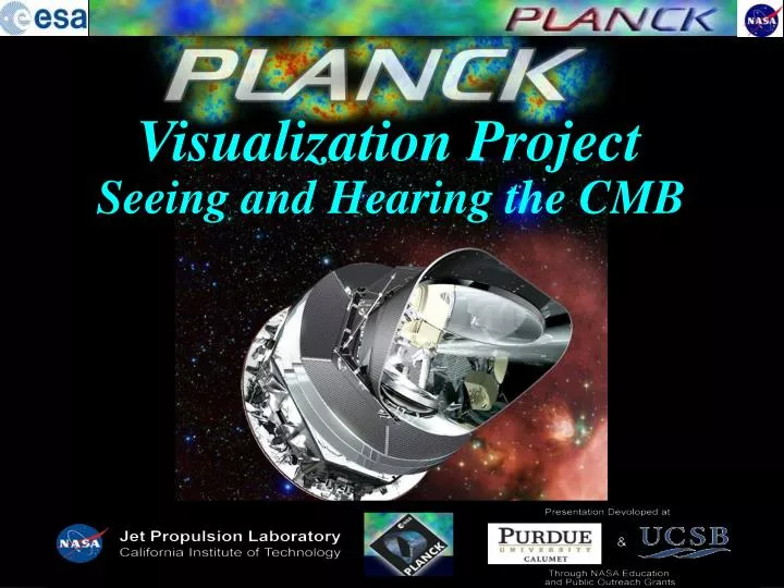
Visualization Project Seeing and Hearing the CMB

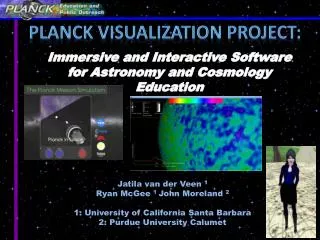
Planck Visualization Project Education and Public Outreach Group, Planck Mission, NASA: University of California, Santa Barbara: Department of Physics Jatila van der Veen (formerly at Purdue-Cal.) Philip Lubin UCSB AlloSphere JoAnn Kuchera-Morin, AlloSphere Director Lead Application Developers: Wesley Smith and Basak Alper, Ph.D. candidates in Media Arts Technology Matt Wright, Media Systems Engineer Purdue University: Purdue-Calumet, VisLab Lead Application Developers: Jerry Dekker, Lead Programmer John “Jack” Moreland, Visualization Specialist Haverford College Bruce Partridge, Friend of the Project Lead P.I., Planck Visualization Project: Jatila van der Veen Planck Project Scientist and Lead Principal Investigator at NASA/JPL: Charles R. Lawrence Planck Launch: May 14, 2009 photo: Charles R. Lawrence

Organization of this presentation: 1. About the Planck Mission and CMB Research 2. Planck in Virtual Reality 3. Understanding the CMB through Music

Planck is a Mission led by the European Space Agency, with significant participation by NASA. Planck’s purpose is to map the Cosmic Microwave Background radiation (or CMB) - the oldest light we can detect - with a sensitivity of a few millionths of a degree Kelvin, and an angular resolution as fine as 5 arc minutes on the sky. This is equivalent to being able to detect the heat of a rabbit on the Moon from the distance of the Earth, and resolve a bacterium on top of a bowling ball!

The CMB is all around us, bathing the Earth, filling all of the visible Universe! 5

The CMB originated at the time when the universe first became cool enough so as to be transparent to electromagnetic radiation, approximately 380,000 years after the Big Bang. The CMB is like a wall of fog that we can’t see behind... oldest light youngest 6

A condensed slice through spacetime: opaque transparent CMB wall Image credit: www.firstgalaxies.org/the-early-universe

Although the early universe was bright and hot, the CMB signal is observed today as microwaves, invisible to human eyes, due to the stretching of space over the past 14 billion years. CMB Image credit: http://mail.jsd.k12.ca.us/bf/bflibrary/images/electromagnetic-spectrum.jpg

To a first order, the CMB is uniform, and follows a perfect black body thermal radiation curve which peaks at 2.725 Kelvin. This temperature corresponds to a wavelength of light of 2 mm, or microwave radiation. An observed temperature difference across the sky of a few parts in 1,000 is not part of the CMB, but an artifact of our motion through the cosmos. Because of our net motion through space, the sky temperature appears slightly warmer in the direction in which we are moving, and slightly cooler in the direction from which we are coming. warmer cooler 9

In 1992 the COBE satellite revealed small variations in the CMB for the first time, all across the sky, which are independent of the motion of the Earth through space. COBE’s instruments were sensitive to few parts in 100,000 in temperature, and had a spatial resolution of 70 of arc on the sky. Called anisotropies, meaning deviations from uniformity, these small temperature variations that we observe in the CMB today are the light echoes of variations in the distribution of matter and energy in the early universe, which acted as ‘seeds’ for galaxies to form later on, by gravitational attraction. COBE all-sky map The CMB anisotropies give us a picture of the Last Scattering Surface of the expanding universe, seen at one moment in time – when matter and radiation first separated. Observing the CMB anisotropies with a sensitivity of a few parts in 100,000 is like measuring centimeter-height ripples on the surface of the ocean as seen from an airplane, a few kilometers above the ground. 10

For reference, 10 of arc on the sky is approximately equal to the width of your pinky, held at arm’s length. A patch of 5 arc minutes on a side is approximately 6 billionths of the total area of the sky. 11

Since the 1980’s, numerous balloon-borne and ground-based experiments have mapped portions of the sky at increasingly fine resolution, but only two previous satellites, COBE and WMAP, have successfully mapped the entire sky. This figure compares the resolution with which COBE and WMAP have been able to map the CMB, with that expected from Planck. 1989 2000 May 14, 2009

How will Planck complete its mission of mapping the CMB at such fine resolution? Primary mirror, 1.9 x 1.5 meters Secondary mirror 1.1 x 1.0 meter The Planck spacecraft is 4.2 m high and has a maximum diameter of 4.2 m, with a launch mass of around 1.8 tons. The spacecraft comprises a service module, which houses systems for power generation and conditioning, attitude control, data handling and communications, together with the warm parts of the scientific instruments, and a payload module. The payload module consists of the telescope, the optical bench, with the parts of the instruments that need to be cooled - the sensitive detector units - and the cooling systems. 13

Planck was built by an international industrial team. Different components, including the mirrors, instruments, payload package, and cooling systems were built in France, Austria, Germany, Denmark, Finland, Belgium, Italy, Ireland, the Netherlands, Norway, Portugal, Spain, Sweden, Switzerland, the United Kingdom, and the United States. 14

Planck will measure the temperature of the sky across 9 frequency channels. HFI (High frequency Instrument): an array of microscopic temperature sensors called spider web bolometers, cooled to 0.1 K LFI (Low frequency Instrument): an array of radio receivers using high electron mobility transistor mixers, cooled to 20 K. HFI feed horn array LFI feed horn array 15

Peak frequency response for each detector, compared with the sky signals HFI LFI 44 70 100 143 30 857 217 353 545

Expected maps of the sky at each frequency: 17

What do we expect to learn from the data? From the accurate temperature maps, we will be able to calculate the Power Spectrum of the anisotropies of the CMB extremely accurately. From a careful analysis of this power spectrum, we expect to derive important characteristic properties of the Universe, and resolve questions in fundamental physics. map power spectrum fundamental physics 18

What techniques do we use to extract information from these data sets? Planck is measuring the microKelvin fluctuations in temperature which are translated into slightly stretched (red shifted) and compressed (blue shifted) fluctuations in microwave radiation. From these microwave fluctuations, we infer pressure differences in the universe at the time that matter and radiation first separated. These pressure differences indicate lumpiness in the distribution of matter and radiation at the time that matter and energy first separated – the CMB. The power spectrum of the CMB tells us the sizes of the lumps in the early universe. We analyze the power spectrum of the CMB using techniques that we know from the physics of MUSIC. slide adapted from Mark Whittle more on this subject later...

Planck will also map the polarization of the CMB Mapping the polarization of the CMB will give us an idea of how photons scattered off charged particles on the Last Scattering Surface. This will give us a picture of the distribution of matter in the universe at that time – similar to the way in which sunlight scatters off the surface of a lake reflects the undulations in the surface of the water. 20

Next: Educational materials that the Planck E/PO Group is developing

The Planck Mission in Virtual Reality Under development at Purdue University Jerry Dekker, Jack Moreland, Jatila van der Veen

Utilizing state-of-the-art visualization, gaming, and distributed computing technology, we are developing applications for the Planck Mission using Virtual Reality to reach the widest possible international audience.

Starting from a flight simulator screen ...

...the user can explore the mission from launch... to orbital insertion... to data gathering operations... from any vantage point in the solar system.

Finally, the user stands “in space” while Planck paints the CMB all around, beyond the starry background.

Simulation created in the Visualization Laboratory at Purdue University-Calumet On May 14, 2009, at 13:12 UT, Planck was launched from the European Space Agency’s launch pad in Kouru, French Guiana.

Distribution goals: • Hi-tech visualization facilities: • VR facilities • Planetaria • Virtual Classrooms • Museums and Science Centers • Thousands of potential sites! • DVDs for Museums and mass dist. • Kiosk interactive display • Passive viewing as movie • Web Distribution • Download, single computer • Interactive served application • Computers in classrooms Currently still in development and testing. If you wish to receive a copy to test, please send an email to jatila@physics.ucsb.edu. • Popular Culture • iPhone application • Google Universe • Screen savers Available in a variety of 3-D technologies, from simple anaglyph to high-tech varieties.

The Music of the Cosmos Using sound to explain how we extract information about the early universe from the power spectrum of the CMB. primordial Planck WMAP COBE Under development at UC Santa Barbara Jatila van der Veen JoAnn Kuchera-Morin Wesley Smith, Basak Alper, Matt Wright

The variations in temperature that we observe in the CMB ... ...tell us about variations in density in the early universe, which we now observe as... ... anisotropies in the CMB. The CMB anisotropies originate from two different processes : Initial distortions in the actual shape of the Universe, which originated in the first moments of its existence Gravity-driven pressure waves in the matter-radiation fluid which filled the young universe during the first 380,000 years of its existence – up to the time when matter and radiation separated.

Those gravity-driven pressure waves in the matter-radiation fluid of the early universe not only left their imprints in the light of the CMB; they determined the distribution of matter and energy in the universe at later times, as seen in the large-scale clusters and walls of galaxies. Images courtesy of Professor Max Tegmark, MIT

That is why it is so important to understand the scale of anisotropies in the CMB: the variations in the oldest light of the universe predict the distribution of matter and energy throughout the universe. This includes “normal” matter, in the form of galaxies that emit radiation, “exotic” dark matter, which gravitates but does not shine, and the stranger still dark energy. In a sense, understanding the CMB is like deciphering the genetic code of the universe!

Measuring and analyzing the CMB is based on the same principles which are involved in making music and broadcasting it! Pressure waves (sounds) in the concert hall are converted to electromagnetic radiation, transmitted across spacetime, and reconverted to sound waves that your ears can hear. Similarly, pressure waves in the early universe resulted in variations in the light that was emitted as radiation and matter decoupled. This light has been transmitted across spacetime (nearly 14 billion years!) to our microwave detectors. Using techniques that are familiar to sound engineers, we can convert these light echoes into to sound that your ears can hear.

In order to understand how we can listen to the sounds of the early universe, we first need to understand how sounds are produced on Earth. Sound waves are just pressure waves which have wavelengths and frequencies that we can hear. Humans can hear frequencies from around 20 to 20,000vibrations/second (Hertz). Figures adapted from Mark Whittle, University of Virginia The frequency, or number of vibrations per second, determines the pitch of the sound we hear. Higher frequency = more vibrations/sec = higher pitch.

Higher frequency waves have shorter wavelengths, and lower frequency waves have longer wavelengths, as indicated in these pictures. Frequency and wavelength are related by the speed of sound by the following equation: Wave speed = frequency x wavelength Thus if you know the speed of sound and the frequency, you can calculate wavelength. The speed of sound in air is approximately 330 meters/second. So… The “red tone” of 200 Hz has a wavelength of 330 m/sec / 200 Hz = 1.65 meters. The “cyan tone” of 600 Hz has a wavelength of 330 m/sec / 600 Hz = 0.55 meters or 55 cm. The “magenta tone” of 1000 Hz has a wavelength of 330 m/sec / 1000 Hz = 0.33 meters or 33 cm.

The amplitude of the pressure variations determines the loudness of the sounds we hear. Higher amplitude = greater variation in pressure = louder sound. Figure adapted from Mark Whittle, University of Virginia The temperature variations of the CMB indicate pressure variations of a few parts in 10,000, or ΔP/P of 10-4 = 110 db, approximately the volume of a typical rock concert.

Finally, we need to understand how instruments produce pleasing sounds: To produce musical tones, you need an object with a well-defined shape and size, which can vibrate – a RESONATOR. Resonators – such as flutes, guitars, drums, or bells - have a fundamental tone which is the longest wavelength that can fit within the walls of a given resonator. The fundamental is the lowest pitch that a given resonator can produce. Higher harmonics are whole number multiples of the fundamental frequency. The fundamental frequency tells you the time it takes for the longest wave to travel across the resonator and back one time.

Bigger resonators produce lower tones. Click on the speaker icons to hear music produced by pressure waves vibrating in each of these wind instruments. Bag pipe Pipe organ Wooden flute Next we’ll investigate the sound waves produced by a computer, by real instruments, and by a star such as the Sun. Finally, we’ll apply these concepts to understanding the sounds produced by pressure waves in the early universe.

The simplest sound wave one can imagine is just a single pure tone, with only one frequency, corresponding to a single wavelength. The top figure shows this tone as a single frequency wave, with a period of 1/440th of a second, or .002273 second. wavelength Click on the speaker to hear a pure “A” of 440 Hz, generated by a computer: The POWER SPECTRUM of any sound tells you what frequencies are present and how loud each one is. Here is the power spectrum of this tone: a single peak at a frequency of 440 Hertz, or cycles/second: 39

Here are 3 A’s, an octave apart: 220 Hz, 440 Hz, and 880 Hz. In the top figure, we display the wave form, which is the superposition of the three waves, and in the bottom figure we display the power spectrum of this sound, comprised of these three notes. The power spectra and wave forms shown on these pages were produced using the software “Cool Edit Pro” Click on the speaker to hear the tones. 220 440 880 40

Here is the sound of a clarinet playing an A of 440 Hz. Notice that even though only one note is being played, the wave form and power spectrum are more complicated than those of an A being played by a computer! This is because the way the pressure waves bounce around inside the actual clarinet creates higher harmonics, or overtones, and it is the overtones which allow you to distinguish one instrument from another, and notes played by real instruments from the same notes synthesized by a computer! Compare the sound of the clarinet (above) playing an A of 440 Hertz, with the sound of a pure A played on a computer: 41

And here is the power spectrum of the clarinet playing an A of 440 Hz. The first peak is the fundamental, at 440 Hz. The successive peaks represent the higher harmonics, which are integer multiples of the fundamental. Compare the spectra and sounds of the real clarinet and the synthesized sound generated by a computer. Clarinet playing an A etc... 440 Hz 880 1320 Pure A synthesized on a computer has only one peak at 440 Hz. 42

Let’s compare the sound of a trumpet playing a middle C (261 Hz) with the same note, synthesized on a computer. Here are the wave forms: Trumpet Source: http://www.ugcs.caltech.edu/~tasha/ Computer 43

And here are the power spectra. Again, notice the higher harmonics are multiples of the fundamental. The presence of these higher harmonics allows you to tell that this note is played by a trumpet. Trumpet etc... 261 783 522 Pure C synthesized on a computer. Notice a single peak at 261 Hz. The absence of the higher harmonics makes this note sound artificial! 44

The point of all this is to demonstrate that although instruments may play the same pitch at the same loudness, each instrument (resonator) has a unique POWER SPECTRUM which is determined by the size and shape of that instrument. The power spectrum, consisting of the fundamental and higher harmonics, is what gives each instrument its unique sound quality (which musicians call TIMBRE), and allows us to distinguish the sound of a piano from that of a violin, trumpet, clarinet, or a tone produced by a computer. A power spectrum is thus a bit like a finger print. Clarinet Trumpet Before we apply these principles to the CMB, we have to look at one little problem: Poor resonators produce “noisy” power spectra, with poorly-defined peaks. The universe was a poor resonator, since it had no well-defined boundaries in space, thus we have to know how to “clean up” a power spectrum before we can listen to the music of the cosmos!

If there is a fair amount of “hiss” in a resonating system, it can be difficult to pick out the peaks – the fundamental and higher harmonics – in the power spectrum. For example: Here’s our piper, playing one note : It is difficult to find the fundamental in this power spectrum, but with mathematical tools called Fourier analysis (after the fellow who invented them) we can remove the hiss and pick out the fundamental tone.

Here is the bag pipe again, but with its power spectrum “cleaned up” to pick out the harmonics from the noise. We hear the fundamental, but the tone has lost its breathy quality, so that it no longer sounds like a bag pipe. Now we have are ready to analyze the sounds of natural systems, starting with the Sun, and then the universe!

Natural systems such as the Sun and the Earth are also resonators. The Sun, being a ball of gas without well defined boundaries, produces very hissy sounds, like these, which have been compressed by several orders of magnitude so as to be audible to human ears: Source: bison.ph.bham.ac.uk/ ~420 Hz 100 Hz 1,000 Hz 10 Hz 48

Using the same Fourier analysis, we can clean up the Sun’s power spectrum and pick out the fundamental and higher harmonics which are buried in all the hiss. With the hiss removed, and scaled to audible frequencies, the Sun would sound something like this: ... Sounds pretty eerie, doesn’t it!

Finally: Back to the CMB! The early universe was a resonator, albeit a very hissy one, like the Sun. Thus it should have a fundamental tone which was determined by the size of the universe at the time that the CMB was produced – when matter and radiation first separated. We can determine the wavelength of the fundamental from the power spectrum of the CMB, and knowing the approximate speed of sound in the early universe, we can calculate the fundamental frequency. We can clean up the power spectrum, scale the frequencies to the range of human hearing, and listen to the sounds of the early universe!

Visualization Project