Turbulence Characteristics in Flow Dynamics
160 likes | 258 Views
Explore the nature of turbulence, from Reynolds numbers to dynamic stability concepts. Learn about turbulent fluxes and vertical transports in fluid flow. Study various models and definitions related to turbulent fluxes in different flow conditions.

Turbulence Characteristics in Flow Dynamics
E N D
Presentation Transcript
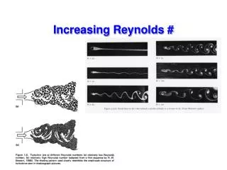
Turbulence characteristics 3-dimensional rotational – carries vorticity (unlike linear surface waves) irregular, unpredictable (random) motion – described by probability density function diffusive – several orders of magnitude greater than molecular diffusion dissipative – K.E.→ heatrequires steady supply of energy
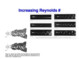
Turbulence characteristics flow has large Reynolds #,(nonlinear) does not obey a dispersion relation (not wavelike) broad wavenumber spectrum generally anisotropic at larger scales is a function of the flow, not the fluid satisfies Navier-Stokes equations
Dynamic Stability Concepts Figure from Thorpe Statically stable, dynamically unstable = forced convection (figure from Stull)
Vertical turbulent transports What is a turbulent flux? Reynolds’ decomposition: <wT> = <w><T> + <w’T’> What determines the vertical distribution of turbulence? TKE equation: dTKE/dt = production – dissipation + advection How does turbulence determine the interfacial fluxes of heat, moisture and momentum? Near-surface gradients and TKE levels are related. How are vertical turbulent transports modeled? Flux profile relationships (Monin-Obukhov similarity theory) closure schemes (parameterizations) layered versus level models
Turbulent Flux Definitions Reference Lecture 2 for bulk parameterizations of these
PBL TKE budget forced convection free convection • u* friction velocity • w* convective velocity scale • h boundary layer height • ε dissipation of TKE • S shear production of TKE • B buoyancy production/damping of TKE • T transport of TKE
the flow is in steady state, i.e, • the boundary layer is horizontally homogeneous, i.e., and • the boundary layer is statically neutral, i.e., • the boundary layer is barotropic, i.e., Ug and Vg are constant with height • there is no subsidence, i.e., W = 0 Ekman Flow assumptions
(1) • How can we solve equation set (1)? • First, let's define the magnitude of the geostrophic wind, G by G = [U2g + V2g]0.5 • Let's also assume that the geostrophic wind is parallel to the X axis, thus: • G = Ug • V2g = 0 • Let's also use first-order local closure K-theory, assuming a constant Kmto eliminate the flux terms. • Hence: (2) • Substituting (2) into (1) gives: • (3) Ekman Flow
Here we have a set of two partial differential equations...., how to solve????? • Well, we need to specify the boundary conditions: • U= 0 at z = 0 • V= 0 at z = 0 • U --> G as z --> large (get above the boundary layer) • V --> 0 as z --> large (the geostrophic flow above the boundary layer is parallel to the X axis) • The solution to (3) using the above boundary conditions is: • (4) • where Ekman Flow