Reynolds Experiment
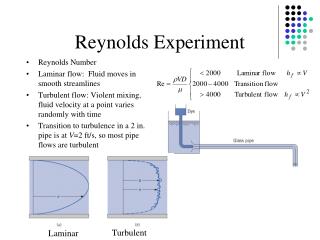
Reynolds Experiment. Reynolds Number Laminar flow: Fluid moves in smooth streamlines Turbulent flow: Violent mixing, fluid velocity at a point varies randomly with time Transition to turbulence in a 2 in. pipe is at V =2 ft/s, so most pipe flows are turbulent. Turbulent. Laminar.

Reynolds Experiment
E N D
Presentation Transcript
Reynolds Experiment • Reynolds Number • Laminar flow: Fluid moves in smooth streamlines • Turbulent flow: Violent mixing, fluid velocity at a point varies randomly with time • Transition to turbulence in a 2 in. pipe is at V=2 ft/s, so most pipe flows are turbulent Turbulent Laminar
Shear Stress in Pipes • Steady, uniform flow in a pipe: momentum flux is zero and pressure distribution across pipe is hydrostatic, equilibrium exists between pressure, gravity and shear forces • Since h is constant across the cross-section of the pipe (hydrostatic), and –dh/ds>0, then the shear stress will be zero at the center (r = 0) and increase linearly to a maximum at the wall. • Head loss is due to the shear stress. • Applicable to either laminar or turbulent flow • Now we need a relationship for the shear stress in terms of the Re and pipe roughness
Darcy-Weisbach Equation Darcy-Weisbach Eq. Friction factor
Laminar Flow in Pipes • Laminar flow -- Newton’s law of viscosity is valid: • Velocity distribution in a pipe (laminar flow) is parabolic with maximum at center.
Nikuradse’s Experiments • In general, friction factor • Function of Re and roughness • Laminar region • Independent of roughness • Turbulent region • Smooth pipe curve • All curves coincide @ ~Re=2300 • Rough pipe zone • All rough pipe curves flatten out and become independent of Re Rough Smooth Blausius OK for smooth pipe Laminar Transition Turbulent
Fully developed flow region Entrance length Le Pressure Entrance pressure drop Region of linear pressure drop x Pipe Entrance • Developing flow • Includes boundary layer and core, • viscous effects grow inward from the wall • Fully developed flow • Shape of velocity profile is same at all points along pipe
Entrance Loss in a Pipe • In addition to frictional losses, there are minor losses due to • Entrances or exits • Expansions or contractions • Bends, elbows, tees, and other fittings • Valves • Losses generally determined by experiment and then corellated with pipe flow characteristics • Loss coefficients are generally given as the ratio of head loss to velocity head • K – loss coefficent • K ~ 0.1 for well-rounded inlet (high Re) • K ~ 1.0 abrupt pipe outlet • K ~ 0.5 abrupt pipe inlet Abrupt inlet, K ~ 0.5
Elbow Loss in a Pipe • A piping system may have many minor losses which are all correlated to V2/2g • Sum them up to a total system loss for pipes of the same diameter • Where,
EGL & HGL for Losses in a Pipe • Entrances, bends, and other flow transitions cause the EGL to drop an amount equal to the head loss produced by the transition. • EGL is steeper at entrance than it is downstream of there where the slope is equal the frictional head loss in the pipe. • The HGL also drops sharply downstream of an entrance