Load Shedding in a Data Stream Manager

1. Load Shedding in a Data Stream Manager Kevin Hoeschele Anurag Shakti Maskey

2. Overview • Loadshedding in Streams example • How Aurora looks at Load Shedding • The algorithms Used by Aurora • Experiments and results

3. Load Shedding in a DSMS • Systems have a limit to how much fast data can be processed • When the rate is too high, Queues will build up waiting for system resources • Loadshedding discards some data so the system can flow • Different from networking loadshedding • Data has semantic value in DSMS • QoS can be used to find the best stream to drop

4. Hospital - Network • Stream of free doctors locations • Stream of untreated patients locations, their condition (dieing, critical, injured, barely injured) • Output: match a patient with doctors within a certain distance Patients Doctors who can work on a patient Join Doctors

5. Too many Patients, what to do? • Loadshedding based on condition • Official name “Triage” • Most critical patients get treated first • Filter added before the Join • Selectivity based on amount of untreated patients Patients Condition Filter Doctors who can work on a patient Join Doctors

6. Aurora Overview • Push based data from streaming sources • 3 kinds of Quality of Service • Latency • Shows utility drop as answers take longer to achieve • Value-based • Shows which output values are most important • Loss-tolerance • Shows how approximate answers affect a query

7. Loadshedding Techniques • Filters (semantic drop) • Chooses what to shed based on QoS • Filter with a predicate in which selectivity = 1-p • Lowest utility tuples are dropped • Drops (random drop) • Eliminates a random fraction of input • Has a p% chance of dropping each incoming tuple

8. 3 Questions of Load Shedding • When • Load of system needs constant evaluation • Where • Dropping as early as possible saves most resources • Can be a problem with streams that fan out and are used by multiple queries • How much • the percent for a random drop • Make the predicate for a semantic drop(filter)

9. Load Shedding in Aurora • Aurora Catalog • Holds QoS and other statistics • Network description • Loadshedder monitors these and input rates: makes loadshedding decisions • Inserts drops/filters into the query network, which are stored in the catalog Load Shedder Changes to Query plans Network description Data rates Catalog Query Network Input streams output

10. Equation • N= network • I=input streams • C=processing capacity • Uaccuracy= utility from loss-tolerance QoS graph • H=Headroom factor, % of sys resources that can be used at a steady state If (Load(N(I)) > C then load shedding is needed (why no H) Goal is to get a new network N’ based on N but where: min{Uaccuracy(N(I))-Uaccuracy(N’(I))} and (Load(N’(I)) < H * C

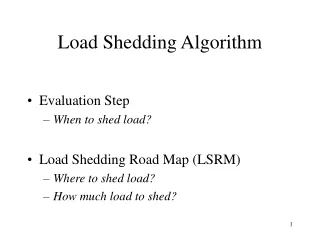
11. Load Shedding Algorithm • Evaluation Step • When to shed load? • Load Shedding Road Map (LSRM) • Where to shed load? • How much load to shed?

12. L = c1 s1 c2 s2 cn sn … I O Load Evaluation • Load Coefficients (L) • the number of processor cycles required to push a single tuple through the network to the outputs • n operators • ci = cost • si = selectivity

13. L2 = 14 L3 = 5 2 c2 = 10 s2 = 0.8 3 cn = 5 sn = 1.0 O1 L1 = 22 1 c1 = 10 s1 = 0.5 I L4 = 10 4 c2 = 10 s2 = 0.9 L(I) = 22 O2 Load Evaluation Load Coefficient L1 = 10 + (0.5 * 10) + (0.5 * 0.8 * 5) + (0.5 * 10) = 22 L2 = 10 + (0.8 * 5) = 14

14. S = Load Evaluation • Stream Load (S) • load created by the current stream rates • m input streams • Li = load coefficient • ri = input rate

15. L2 = 14 L3 = 5 2 c2 = 10 s2 = 0.8 3 cn = 5 sn = 1.0 O1 L1 = 22 1 c1 = 10 s1 = 0.5 I L4 = 10 4 c2 = 10 s2 = 0.9 L(I) = 22 O2 r = 10 Load EvaluationStream Load S = 22 * 10 = 220

16. Load Evaluation • Queue Load (Q) • load due to any queues that may have built up since the last load evaluation step • MELT_RATE = how fast to shrink the queues (queue length reduction per unit time) • Li = load coefficient • qi = queue length Q = MELT_RATE * Li * qi

17. L2 = 14 L3 = 5 q = 100 2 c2 = 10 s2 = 0.8 3 cn = 5 sn = 1.0 O1 L1 = 22 1 c1 = 10 s1 = 0.5 I L4 = 10 4 c2 = 10 s2 = 0.9 L(I) = 22 O2 r = 10 Load EvaluationQueue Load MELT_RATE = 0.1 Q = 0.1 * 5 * 100 = 50

18. L2 = 14 L3 = 5 q = 100 2 c2 = 10 s2 = 0.8 3 cn = 5 sn = 1.0 O1 L1 = 22 1 c1 = 10 s1 = 0.5 I L4 = 10 4 c2 = 10 s2 = 0.9 L(I) = 22 O2 r = 10 Load EvaluationTotal Load • Total Load (T) = S + Q T = 220 + 50 = 270

19. T > H * C processing capacity headroom factor Load Evaluation • The system is overloaded when

20. Load Shedding Algorithm • Evaluation Step • When to drop? • Load Shedding Road Map (LSRM) • How much to drop? • Where to drop?

21. how many cycles will be saved <Cycle Savings Coefficients (CSC) Drop Insertion Plan (DIP) Percent Delivery Cursors (PDC)> set of drops that will be inserted where the system will be running when the DIP is adopted ENTRY 1 … … … ENTRY n CSC DIP PDC max savings … (0,0,0,…,0) cursor less load shedding more load shedding Load Shedding Road Map (LSRM)

22. set Drop Locations compute & sort Loss/Gain ratios Drop-Based LS Filter-Based LS take the least ratio take the least ratio how much to drop? how much to drop? insert Drop determine predicate create LSRM entry insert Filter create LSRM entry LSRM Construction

23. set Drop Locations compute & sort Loss/Gain ratios Drop-Based LS Filter-Based LS L1 = 17 L2 = 14 L3 = 5 1 c1 = 10 s1 = 0.5 2 c2 = 10 s2 = 0.8 3 cn = 5 sn = 1.0 O I A B C D Drop Locations Single Query

24. set Drop Locations compute & sort Loss/Gain ratios Drop-Based LS Filter-Based LS L1 = 17 L2 = 14 L3 = 5 1 c1 = 10 s1 = 0.5 2 c2 = 10 s2 = 0.8 3 cn = 5 sn = 1.0 O I A Drop Locations Single Query

25. set Drop Locations compute & sort Loss/Gain ratios Drop-Based LS Filter-Based LS L2 = 14 L3 = 5 2 c2 = 10 s2 = 0.8 3 cn = 5 sn = 1.0 D E O1 B L1 = 22 1 c1 = 10 s1 = 0.5 A I L4 = 10 C 4 c2 = 10 s2 = 0.9 F O2 Drop Locations Shared Query

26. set Drop Locations compute & sort Loss/Gain ratios Drop-Based LS Filter-Based LS L2 = 14 L3 = 5 2 c2 = 10 s2 = 0.8 3 cn = 5 sn = 1.0 O1 B L1 = 22 1 c1 = 10 s1 = 0.5 A I L4 = 10 C 4 c2 = 10 s2 = 0.9 O2 Drop Locations Shared Query

27. set Drop Locations compute & sort Loss/Gain ratios Drop-Based LS Filter-Based LS utility 1 0.7 0 % tuples 100 50 0 Loss/Gain RatioLoss • Loss – utility loss as tuples are dropped – determined using loss-tolerance QoS graph Loss for first piece of graph = (1 – 0.7) / 50 = 0.006

28. set Drop Locations compute & sort Loss/Gain ratios Drop-Based LS Filter-Based LS Gain G(x) = Loss/Gain RatioGain • Gain – processor cycles gained • R = input rate into drop operator • L = load coefficient • x = drop percentage • D = cost of drop operator • STEP_SIZE = increments for x to find G(x)

29. Drop-Based LS take the least ratio how much to drop? insert Drop create LSRM entry Drop-Based Load Sheddinghow much to drop? • Take the least Loss/Gain ratio • Determine the drop percentage p

30. Drop-Based LS take the least ratio how much to drop? insert Drop create LSRM entry L1 = 17 L2 = 14 L3 = 5 1 c1 = 10 s1 = 0.5 2 c2 = 10 s2 = 0.8 3 cn = 5 sn = 1.0 O I A drop drop drop drop Drop-Based Load Sheddingwhere to drop? If there are other drops in the network, modify their drop percentages.

31. Drop-Based LS take the least ratio how much to drop? insert Drop create LSRM entry Drop-Based Load Sheddingmake LSRM entry • All drop operators with the modified percentages form the DIP • Compute CSC • Advance QoS cursors and store in PDC LSRM Entry <Cycle Savings Coefficients (CSC) Drop Insertion Plan (DIP) Percent Delivery Cursors (PDC)>

32. Filter-Based LS take the least ratio how much to drop? determine predicate insert Filter create LSRM entry Filter-Based Load Sheddinghow much to drop?predicate for filter • Start dropping from the interval with the lowest utility. • Keep a sorted list of intervals according to their utility and relative frequency. • Find out how much to drop and what intervals are needed to . • Determine the predicate for filter.

33. Filter-Based LS take the least ratio how much to drop? determine predicate insert Filter create LSRM entry L1 = 17 L2 = 14 L3 = 5 1 c1 = 10 s1 = 0.5 2 c2 = 10 s2 = 0.8 3 cn = 5 sn = 1.0 O I A filter filter filter filter Filter-Based Load Sheddingplace the filter If there are other filters in the network, modify their selectivities.

34. Experiment setup • Simulated network • Processing tuple time simulated by having the simulator process use the cpu for amount of time needed for an operator to consume a tuple • Process for each input stream • randomly created network • Num querys, Num operations for querys chosen • Random networks a good benchmark?

35. Experiments • Used only Join, Filter, Union Aurora Operators • Filters were simple comparison predicates of the form: • Input_value > filter_constant • Filters and Drops loadshedding were Compared to 4 Admission Control Algorithms • Similar in style to networking loadshedding

36. Evaluation Methods • Loss-tolerance, and Value-based QoS were used • Tuple Utility is the utility from Loss-tolerance QoS • K= num time segments • ni= num tuples per time segment i • ui= loss-tolerance utility for each tuple during time segment i

37. Value Utility • Value Utility is the Utility from value-based QoS • fi= relative frequency of tuples in value interval i with no drops • fi’=frequency relative to the total number of tuples • Ui=average value utility for value interval i • When there are multiple queries, Overall Utility is the sum of the utilities for each query

38. Algorithms • Input-Random • One random stream is chosen, and tuples are shed untill excess load is covered • if the whole stream is shed and there is still excess load, another random stream is chosen • Input-Cost-Top • Similar to Input-Random, but uses the input stream with the most costly input • Input-Uniform • Distributes load shedding uniformly by each input stream • Input-Cost-Uniform • Load is shed of all input streams, weighted by their cost

39. Results – Tuple Utility Loss Observations: QoS driven Algorithms Perform better Filter works better then Drop

40. Results -Value utility loss Filter-LS is clearly the best Drop-LS is no better then the Admission control algorithms

41. Conclusion • Loadshedding is important to DSMS • Many variables to considor when planning to use Loadshedding • Drop and Filter are two QoS driven algorithms • QoS based strategies work better then Admission control

42. Questions • Drop and Filter were the two QoS loadshedding algorithms given here. Are there any others? • Admission Control may be a viable option in processing network requests, but in a streaming database system the connection is already made. Where putting the incoming tuples into a buffer to in effect deny the stream bandwidth, would this increase utility? • Why are REDs useful or not useful for streaming databases?

43. More Questions • When we have a low bandwidth connection like a sensor that is unreliable and when a significant amount of traffic is out of order, is TCP the best transport protocol? • When there is high traffic, to what extent should the network do the load shedding? Should the database system be doing more because it knows the semantics of the tuples? • So the idea of Admission control doesn't directly cross-over from networks to streaming databases.  But does the idea of buffering the input when the process becomes overloaded, achieve the same effect?  Why doesn't aurora have this?