EART20170 data analysis lecture 7: Correlation, regression and error propagation

1. EART20170 data analysislecture 7: Correlation, regression and error propagation Dr Paul Connolly

2. Intended learning outcomes • Know how to assess how well variations in one variable can be used to explain variations in another. • Fit straight lines and curves to data • Mathematics I am afraid! • Test the hypothesis that your correlation coefficients are real. • Error propagation.

3. Definitions • The sample correlation coefficient, • symbol r. • The population correlation coefficient, • symbol r.

4. Definition - correlation coefficient r = +1 r = -1 r = 0 y y y • Some values of r: x x x Perfect positive correlation Perfect negative correlation No correlation Ouch! Good we don’t need to know it MATLAB: corrcoef(x,y) Or corr2(x,y) can be used Excel: =correl(range1,range2)

5. 1.0 0.9 0.8 0.7 0.6 r2, fraction of explained variation 0.5 0.4 0.3 0.2 0.1 0.0 +1.0 +0.5 +0.0 -0.5 -1.0 Correlation coefficient, r Definition - correlation coefficient • r2 is the amount of variation in x and y that is explained by the linear relationship. It is often called the `goodness of fit’ • E.g. if an r = 0.97 is obtained then r2 = 0.95 so 100x0.95=95% of the total variation in x and y is explained by the linear relationship, but the remaining 5% variation is due to “other” causes. It is sometimes important to assess whether the correlation could have occurred by chance => hypothesis test.

6. Methodology: • State the null and alternate hypotheses: • E.g. H0: r=0, H1: r≠0 • Calculate a statistic (to be defined): something that if null hypothesis is true is distributed according to a theoretical distribution. • Calculate a critical value from the theoretical distribution. • Assess which is largest: statistic or critical value and • Accept the null if statistic < critical value or reject the null (and hence accept the alternate) if statistic > critical value.

7. Why does this kind of hypothesis testing work? • Statisticians have found that if you take a random sample of quantitative data, size n, from a population and then another independent sample size n, then calculate the correlation coefficient, r… • will be: • Distributed according to a t-distribution (if the data are drawn from the same population), with n-2 degrees of freedom • Therefore, if we calculate a value of t from our data that is large, we can say it is unusual.

8. One-tailed and two-tailed tests • When testing hypotheses of the correlation coefficient we usually only use the two-tailed test • E.g. CO2 levels vs temperature have a correlation coefficient that is different to 0. • If we take limited data sizes we can get high correlation coefficients.

9. Correlation: CO2 vs temperature Question is, given there is only a small amount of data here, is the correlation coefficient significant?

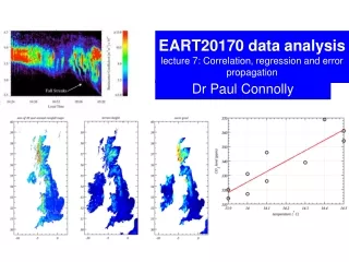
10. Correlation: rain vs terrain:is rainfall correlated to terrain?

11. Does chocolate make you clever?

12. Calculate the correlation coefficient, r, and the standard deviation of y and x Calculate the mean of x and the mean of y Fitting straight lines  could be the heat it takes to heat up the apparatus (e.g. kettle filament, etc).

13. So fitting log of the drop number at time t against t will give a straight line with an intercept of log of N0 and a slope of –J.

14. So fitting log of the terminal velocity against log of diameter D will give a straight line with an intercept of log of a and a slope of b. • Are particles sedimenting due to Stokes’ law: • non turbulent, v=aD2 • or are they in a turbulent flow regime: • v=aD0.5

15. Error propagation

18. Final answer

19. Tomorrows practical: lidar data within clouds that I’ve worked on as part of my research

20. Question was how much water-ice is present in Martian clouds?

21. Data were taken by the Phoenix Lander on Mars The mission responded to evidence returned from NASA's Mars Odyssey orbiter in 2002 indicating that most high-latitude areas on Mars have frozen water mixed with soil within arm's reach of the surface The vertical green line in this illustration shows how the weather station on Phoenix will use a laser beam from a lidar instrument to monitor dust and clouds in the atmosphere.

22. Airborne measurements on Earth Ozonesondes (profiles) ARA Egrett, 10 - 15 km NERC Dornier 0-5 km

23. Sampling method: • Grob Egret: sampled cirrus clouds in-situ. • Measurements: Particle microphysics, turbulence, water vapour, temperature, IR fluxes. • Kingair:remotely sensed cirrus clouds from below by airborne LIDAR.

24. Fly through the clouds with aircraft and sample them Australian clouds… Use regression between measured ice water content to extinction in Earth’s clouds and apply this to Martian clouds.

25. Log of ice water content versus log of extinction is a straight line. Watch out for `base’ of logarithm! Well-trained eye: note that when you see this much data falling close to a straight line, it is pretty clear that the correlation is going to be statistically significant This implies a power law

26. For fitting a power law such as: IWC=AxExtb It could be that you fitted a power law, for example your input was log(x) and log(y) and you fitted a straight line. In this case, after fitting your straight line, you would have to calculate A=exp(a) and b=b