Introduction to the design of cDNA microarray experiments

Introduction to the design of cDNA microarray experiments Statistics 246, Spring 2002 Week 9, Lecture 1 Yee Hwa Yang

Some aspects of design Layout of the array • Which cDNA sequence to print? • Library • Controls • Spatial position Allocation of samples to the slides • Different design layout • A vs B : Treatment vs control • Multiple treatments • Time series • Factorial • Replication • number of hybridizations • use of dye swap in replication • Different types replicates (e.g pooled vs unpooled material (samples)) • Other considerations • Physical limitations: the number of slides and the amount of material • Extensibility - linking

Issues that affect design of array experiments Scientific • Aim of the experiment Specific questions and priorities between them. How will the experiments answer the questions posed? Practical (Logistic) • Types of mRNA samples: reference, control, treatment 1, etc. • Amount of material. Count the amount of mRNA involved in one channel of a hybridization as one unit. • Number of slides available for experiment. Other Information • The experimental process prior to hybridization: sample isolation, mRNA extraction, amplification , labelling. • Controls planned: positive, negative, ratio, etc. • Verification method: Northern, RT-PCR, in situ hybridization, etc.

Graphical representation

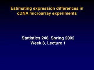
Case 1: Meaningful biological control (C) Samples: Liver tissue from four mice treated by cholesterol modifying drugs. Question 1: Genes that respond differently between the T and the C. Question 2: Genes that responded similarly across two or more treatments relative to control. Case 2: Use of universal reference. Samples: Different tumor samples. Question: To discover tumor subtypes. T2 T3 T4 T1 T2 Tn Tn-1 T1 Ref Natural design choice C

Direct vs Indirect Two samples e.g. KO vs. WT or mutant vs. WT Indirect Direct T Ref T C C average (log (T/C)) log (T / Ref) – log (C / Ref ) 2 /2 22

A B C A A B C C B O O One-way layout: one factor, k levels All pair-wise comparisons are of equal importance

Dye-swap A A C B C B Design B2 Design B1 • - Design B1 and B2 have the same average variance • - The direction of arrows potentially affects the bias • of the estimate but not the variance • For k = 3, efficiency ratio (Design A1 / Design B) = 3 • In general, efficiency ratio = (2k) / (k-1)

Design: how we sliced up the bulb A D P L V M

Multiple direct comparisons between different samples (no common reference) Different ways of estimating the same contrast: e.g. A compared to P Direct = log(A/P) Indirect = log(A/M) + log((M/P) or log(A/D) + log(D/P) or log(A/L) – log((P/L) D A M L P V How do we combine these?

Linear model analysis Define a matrix X so that E(Y)=Xb a = log(A), p=log(P), d=log(D), v=log(V), m=log(M), l=log(L)

Time Series T1 T2 T3 T4 T5 T6 T7 Ref • Possible designs: • All sample vs common pooled reference • All sample vs time 0 • Direct hybridization between times. Pooled reference Compare to T1 t vs t+1 t vs t+2 t vs t+3

T2 T4 T1 T3 T2 T4 T1 T3 T2 T4 T1 T3 Ref T1 T2 T3 T4 T1 T2 T3 T4 T2 T4 T1 T3

2 by 2 factorial – two factors, each with two levels Example 1: Suppose we wish to study the joint effect of two drugs, A and B. 4 possible treatment combinations: C: No treatment A: drug A only. B: drug B only. A.B: both drug A and B. Example 2: Our interest in comparing two strain of mice (mutant and wild-type) at two different times, postnatal and adult. 4 possible samples: C: WT at postnatal A: WT at adult (effect of time only) B: MT at postnatal (effect of the mutation only) A.B : MT at adult (effect of both time and the mutation).

Factorial design m m+a Different ways of estimating parameters. e.g. B effect. 1 = (m + b) - (m) = b 2 - 5 = ((m + a) - (m)) -((m + a)-(m + b)) = (a) - (a + b) = b 2 C A 4 1 3 5 6 B AB m+b m+a+b+ab

C A 2 4 1 3 5 AB B 6 Factorial design m m+a m+a+b+ab m+b

C A C A C A A B A.B A.B A.B B B A.B B C 2 x 2 factorial Table entry: variance

Linear model analysis Define a matrix X so that E(Y)=Xb Use least squares estimate for a, b, ab

A B A.B y2 y3 y1 C y1 = log (A / C) = a y2 = log (B / C) = b y3 = log (AB / C) = a + b + ab Common reference approach Estimate (ab) with y3 - y2 - y1

C A C A C A A B A.B A.B A.B B B A.B B C 2 x 2 factorial Table entry: variance

More general n by m factorial experiment 2 factors, one with n levels and the other with m levels OE experiment (2 by 2): interested in difference between zones, age and also zone.age interaction. Further experiment (2 by 3): only interested in genes where difference between treatment and controls changes with time. treatment control control treatment 0 12 24 0 12 24

WT.P21  + a1 + a2 WT P1  WT.P11  + a1 2 5 7 4 1 MT.P21  + (a1 + a2) + b + (a1 + a2)b MT.P1  + b MT.P11  +a1+b+a1.b 3 6

Replication • Why replicate slides: • Provides a better estimate of the log-ratios • Essential to estimate the variance of log-ratios • Different types of replicates: • Technical replicates • Within slide vs between slides • Biological replicates

Sample size Apo A1 Data Set

Technical replication - labelling • 3 sets of self – self hybridization: (cerebellum vs cerebellum) • Data 1 and Data 2 were labeled together and hybridized on two slides separately. • Data 3 were labeled separately. Data 3 Data 2 Data 1 Data 1

Technical replication - amplification • Olfactory bulb experiment: • 3 sets of Anterior vs Dorsal performed on different days • #10 and #12 were from the same RNA isolation and amplification • #12 and #18 were from different dissections and amplifications • All 3 data sets were labeled separately before hybridization

T1 T2 Replicate Design 1 amplification 1 2 3 4 T1 amplification Replicate Design 2 amplification T2 1 2 3 4 amplification Amplified samples Original samples

M1 = Lc.MT.P1  M2 = Lc.WT.P11  + 1 M3 = Lc.WT.P21  + (1 + 2) M4 = Lc.MT.P1  +  M5 = Lc.MT.P11  + 1 +  + 1 * M6 = Lc.MT.P21  + (1 + 2) +  + (1 + 2)* Common reference approach Estimate (1.) with M5 – M4 - M2 + M1 Estimate (1 + 2). with M6 – M4 – M3 + M1

Introduction to the design of cDNA microarray experiments