
Static Analysis: Reaching Definitions and Available Expressions
E N D
Presentation Transcript
Program Analysis Mooly Sagiv http://www.math.tau.ac.il/~sagiv/courses/pa.html Tel Aviv University 640-6706 Sunday 18-21 Scrieber 8 Monday 10-12 Schrieber 317 Textbook: Dataflow AnalysisKill/Gen Problems Chapter 2
Kill/Gen Problems • A simple class of static analysis problems • Generalizes the reaching definition problem • The static information consist of sets of “dataflow” facts • Compute information on the history/future of computations • Generate a system of equations • Use union/intersection to merge information along different control flow paths • Find minimal/maximal solutions
The Reaching Definitions (Revisited) • RDexit (l) = (RDentry (l) - kill) gen • assignments • kill([x := a]l) ={(x, l’) | l’ Lab*} • gen ([x := a]l)= {(x, l)} • skip • kill([skip]l)= • gen ([skip]l) = • RDentry (l) = {l’ pred(l)}RDexit(l’)
Remark B#RD(RDentry (l) )= (RDentry (l) - kill(l)) gen(l)
Front-End Information (Reaching Definitions) • init(S) -The label that S begins • final(S) - The labels that S end • flow(S) - The control flow graph of S • block(l) -The elementary block associated with l • FV(S) -The variables used in S • S*-The analyzed program
Flow Information in While • init:StmLab* • init([x := a]l)= l • init([skip]l)= l • init(S1 ; S2) = init(S1) • init(if [b]lthen S1else S2) = l • init(while [b]l do S) = l • final:StmP(Lab*) • final([x := a]l)= {l} • final([skip]l)= {l} • final(S1 ; S2) = final(S2) • final(if [b]lthen S1else S2) = final(S1) final(S2) • final(while [b]l do S) = {l}
Flow Information in While • flow:LabP(Lab* Lab*) • flow([x := a]l)= • flow([skip]l)= • flow(S1 ; S2) = flow(S1) flow(S2) {(l, l’) | l final(S1),l’ =init(S2)} • flow(if [b]lthen S1else S2) =flow(S1) flow(S2) {(l, l’) | l’ =init(S1)} {(l, l’) | l’ =init(S2)} • flow(while [b]l do S) = flow(S) {(l, l’) | l’ =init(S)} {(l’, l) | l’ final(S)}
Elementary Blocks in While • [x := a]l • block(l)=[x := a]l • [skip]l • block(l)=[skip]l • [b]l • block(l)=[b]l
The Power Program [z := 1]1; while [x>0]2 do ( [z:= z * x]3; [x := x - 1]4 )
The System of Equations [z := 1]1; while [x>0]2 do ([z:= z * x]3; [x := x - 1]4)
Chaotic Iterations for l Lab*do RDentry(l) := RDexit(l) := RDentry(init(S*)) := {(x, ?) | x FV(S*)} WL= Lab* while WL != do Select and remove an arbitrary l WL if (temp != RDexit(l)) RDexit(l) := temp for l' such that (l,l') flow(S*) do RDentry(l') := RDentry(l') RDexit(l) WL := WL l’
AvailableExpressions • The computation of a complex program expression e at a program point l can be avoided if: • e is computed on every path to l and none of its arguments are changed • e is side effect free • A simple example • e can be savedin a temporary variable/register • For simplicity only consider “formal” expressions [x := a+b]1; [y := a*b]2; while [y >a+b]3 do ( [a:= a + 1]4; x := a+b]5)
The Largest Conservative Solution • It is undecidable to compute the exact available expressions • Compute a conservative approximation • We are looking for a maximal set of available expressions • Example [x := a +b]1 while [true]2 do [skip]3 • Minimal set of “missed” expressions • The problem is a must problem • An expression e is available at l if e must be computed on all the paths leading to l
Front-End Information (Available Expressions) • init(S) -The label that S begins • final(S) - The labels that S end • flow(S) - The control flow graph of S • block(l) -The elementary block associated with l • AExp(S) -The set of formal expressions in S • FV(e) -The variables used in the expression e • S*-The analyzed program
Remark B#AE(AEentry (l) )= (AEentry (l) - kill(l)) gen(l)
An Example [x := a+b]1; [y := a*b]2; while [x>0]3 do ( [z:= z * x]4; [x := x - 1]5 )
Chaotic Iterations for l Lab*do AEentry(l) := AExp(S*) AEexit(l) := AExp(S*) AEentry(init(S*)) := WL= Lab* while WL != do Select and remove an arbitrary l WL if (temp != AExit(l)) AEexit(l) := temp for l' such that (l,l') flow(S*) do AEentry(l') := AEentry(l') AEexit(l) WL := WL l’
Dual Available Expressions • It is possible to compute available expressions representing those expressions that may-not-be available • An expression e is not-available at l if e may-not be computed on some of the paths leading to l • This is may problem • The smallest set is computed
Backward(Future) Data Flow Problems • So far we saw two examples of analysis problems where we collected information about past computations • Many interesting analysis problems we are interested to know about the future • Hard for dynamic analysis!
Liveness Data Flow Problems • A variable x may be live at l if there may be an execution path from l in which the value of x is used prior to assignment • An Example:[x := 2;]1 [y := 4;]2 [x := 1;]3 if [ y>x]4 then [z :=y]5 else [z := y*y]6 [x :=z]7 • Usage of liveness • register allocation • dead code elimination • more precise garbage collection • uninitialized variables
Example [x := 2;]1 [y := 4;]2 [x := 1;]3 if [y>x]4 then [z :=y]5 else [z := y*y]6 [x :=z]7
Chaotic Iterations for l Lab*do LVentry(l) := LVexit(l) := for l final(S*)do LVexit(l) := WL= Lab* while WL != do Select and remove an arbitrary l WL if (temp != LVentry(l)) LVentry(l) := temp for l' such that (l’,l) flow(S*) do LVexit(l') := LVeexit(l') LVentry(l) WL := WL l’
Characterization of Dataflow Problems • Direction of flow • forward • backward • Initial value • Control flow merge • May(union) • Must (intersection) • Solution • Smallest • Largest
Backward (Future)Must ProblemVery Busy Expressions • An expression e is very busy at l if its value at l must be used in all the paths from l • Example programif [a>b]1 then [x :=b-a]2 [y := a-b]3else [y :=b-a]4 [x := a-b]5 • Usage of Very Busy Expressions • Reduce code size • Increase speed • Find the largest solution
Chaotic Iterations for l Lab*do VBntry(l) := AExp(S*) VBexit(l) := AExp(S*) for l final(S*)do VBexit(l) := WL= Lab* while WL != do Select and remove an arbitrary l WL if (temp != VBentry(l)) VBentry(l) := temp for l' such that (l’,l) flow(S*) do VBexit(l') := VBeexit(l') VBentry(l) WL := WL l’
Bit-Vector Problems • Kill/Gen problems are also called Bit-Vector problems • Y = (X - Kill) Gen • Y[i]=(X[i] Kill[i]) Gen[i] • Every component can be computed individually(in linear time)
Non Kill/Gen Problems • truly-live variables • A variable vmay betruly live at l if there may be an execution path to l in which v is (transitively) used prior to assignment in a print statement • May be “garbage” (uninitialized) • A variable v may be garbage at l if there may be an execution path to l in which v is either not initialized or assigned using an expression with occurrences of uninitialized variables
Non Kill/Gen Problems(Cont) • May-points-to • A pointer variable pmay point to a variable q at l if there may be an execution path to l in which p holds the address of q • Sign Analysis • A variable vmust be positive/negative l if on all execution paths to lv has positive/negative value • Constant Propagation • A variable vmust be a constant at l if on all execution paths to lv has a constant value
Conclusions • Kill/Gen Problems are simple useful subset of dataflow analysis problems • Easy to implement