Download

1 / 16
160 likes | 226 Views
Explore innovative visualization techniques for high-dimensional data using functions and diagrams. Discover the concept of Functional-P-trees and their application in data analysis.

E N D
Visualization of High-Dimensional Space Maria Canton, William Perrizo Dept. of CS, North Dakota State University. CATA 2007 – Honolulu, Hawaii
A1 A2 An : : . . . graph(f) = {(a1,...,an,f(a1.an))| (a1..an)R } Y S contour(f,S) R R=A1..An space f YS R* R f A1 A2 An x1 x2 xn : . . . Y f(x) A1 A2 An Af x1 x2 xn f(x) : . . . A 1-D visualization approach is thru functionals: f:R(A1..An)Y (lo dim range). Given S Y (subset of the range), contour(f,S) f-1(S). There isDUALITYbetween functionals, f:R(A1..An)Y and derived attributes, Af of R given by x.Af f(x) where Dom(Af)=Y Contour(Af,S) = SELECT A1..An FROM R* WHERE R*.Af S. If S={a}, f-1({a}) is also called Isobar(f, a)
A1A2A3A4A5 A 2 dimensional visualization approach is through Diagrams (their centroids as functionals also provide another 1D visualization) Intersection points with the vertical lines represent attribute values. Means, shown by 3 dots, are the 1D derived attribute, or functional. Note, red and green centroids are approx. equidistant from blue (whereas the green line is clearly an outlier wrt blue and red) (Parallel Coords do not distinguish the green as an outlier). Parallel Coordinate Diagrams are given as a reference point.
A2 A3 A1 A4 A5 Diagrams (cont.) Jewel 2D diagrams. If the vertical lines are wrapped around a regular n-gon. The centroids (3 dots) are the 1D derived attribute, or functional. Note, still they do not distinguish green as outlier.
A5 A1 Diagrams (cont.) Always Up Grade Himalayan (AUGH) 2-D diagrams. Vertical lines from parallel coords are joined and the angle of inclination is doubled each time. Result, shown by 3 dots, is the derived attribute, or functional. Note, green centroids shows up more clearly as an outlier.
Vertical structures for 1D and 2D Visualizations (P-trees). R( A1 A2 A3 A4) R[A1] R[A2] R[A3] R[A4] 010 111 110 001 011 111 110 000 010 110 101 001 010 111 101 111 101 010 001 100 010 010 001 101 111 000 001 100 111 000 001 100 010 111 110 001 011 111 110 000 010 110 101 001 010 111 101 111 101 010 001 100 010 010 001 101 111 000 001 100 111 000 001 100 Vertical Scan of Horizontal records R11 R12 R13 R21 R22 R23 R31 R32 R33 R41 R42 R43 0 1 0 1 1 1 1 1 0 0 0 1 0 1 1 1 1 1 1 1 0 0 0 0 0 1 0 1 1 0 1 0 1 0 0 1 0 1 0 1 1 1 1 0 1 1 1 1 1 0 1 0 1 0 0 0 1 1 0 0 0 1 0 0 1 0 0 0 1 1 0 1 1 1 1 0 0 0 0 0 1 1 0 0 1 1 1 0 0 0 0 0 1 1 0 0 0 0 0 1 0 01 0 1 0 1 0 0 1 0 0 1 01 1. Whole file is not pure1 0 2. 1st half is not pure1 0 0 0 0 0 1 01 P11 P12 P13 P21 P22 P23 P31 P32 P33 P41 P42P43 3. 2nd half is not pure1 0 0 0 0 0 1 0 0 10 01 0 0 0 1 0 0 0 0 0 0 0 1 01 10 0 0 0 0 1 10 0 0 0 0 0 0 0 1 0 0 0 0 1 10 0 0 0 0 1 1 0 0 0 0 0 0 0 1 0 0 0 0 1 0 1 4. 1st half of 2nd half not 0 0 0 1 0 1 01 5. 2nd half of 2nd half is 1 0 1 0 6. 1st half of 1st of 2nd is 1 Eg, Count occurences of 111 000 001 1000 23-level P11^P12^P13^P’21^P’22^P’23^P’31^P’32^P33^P41^P’42^P’43 =0 0 22-level=2 01 21-level 7. 2nd half of 1st of 2nd not 0 P-trees are vertical structures (slices) processed horizontally (ANDs..) To create P-trees, compress bit slices as: Traditionally, data is structured horizontally(into records) and processed vertically (through scans). R11 0 0 0 0 1 0 1 1 The binary basic P-tree, P1,1, for bit-slice R11 is built top-down by record truth of predicate pure1 recursively on halves, until purity is reached. But it is pure (pure0) so this branch ends
Definition of P-trees based on functionals? Given f:R(A1..An)Y and SY define the uncompressed Functional-P-tree as Pf, S a bit map given by Pf,S(x)=1 iff f(x)S. . The predicate for Pf,S is the set containment predicate, f(x)S Pf,S a Contour bit map (bitmaps, rather than lists contour points). If f is a local density (as in the OPTICS clustering method) and {Sk} a partition of Y, {f-1(Sk)} is a clustering! What partition {Sk} of Y should be use? E.g., binary partition? (given by threshold value) In OPTICS Sks are the intervals between crossing points of graph(f) and a threshold line pts below the threshold line are agglomerated into 1 noise cluster. Weather reporters use equi-width interval partitions (of barametric pressure or temp..).
Singly Compressed Functional-P-trees(with equi-width leaf size, ls) (ls)Pf,S is a compression of Pf,S by doing the following: 1. order or walk R(converts the bit map to a bit vector) 2. equi-width partition R into segments of size, ls(ls=leafsize, last 1 can be short) 2.5. Define E and U, 2 bit vectors of size=#segments: Initialize E to pure 1, U to pure 0. 3. eliminate and mask to 0 in E, all pure-zero segments 4. eliminate and mask to 1 in U, all pure-one segments 1. E is Existential segment mask, U is Universal or Pure1 segment mask (Pure0 mask = E') 2. There can be partitions other than equi-width. 3. (ls)Pf,S is given by E, U and its mixed leaves (only). Doubly Compressed Functional-P-treeswith equi-width leaf sizes, (ls1,ls2)Each leaf of (ls)Pf,S is an uncompressed bit vector and can be compressed same way: (ls1,ls2) Pf,S (ls2 is 2nd equi-width segmentation size and ls2<< ls1) Recursive compression can continue...(ls1,ls2,ls3)Pf,S (ls1,ls2,ls3,ls4) Pf,S...
2xRd=1..nad(k2kxdk) + |R||a|2 = xRd=1..n(k2kxdk)2 - 2xRd=1..nad(k2kxdk) + |R||a|2 = xd(i2ixdi)(j2jxdj) - |R||a|2 = xdi,j 2i+jxdixdj- 2 x,d,k2k adxdk + |R||a|2 |R|dadad = x,d,i,j 2i+j xdixdj- = x,d,i,j 2i+j xdixdj- 2|R| dadd + 2 dadx,k2kxdk + TV(a) = i,j,d 2i+j |Pdi^dj| - k2k+1 dad |Pdk| + |R||a|2 TV(a) = i>j,d 2i+j+1 |Pdi^dj| + k,d (22k- 2k+1ad) |Pdk| + |R| (a12+..+an2) dadad ) = x,d,i,j 2i+j xdixdj+ |R|( -2dadd + The Total Variation Functional aR(A1..An) TV(a)=xR(x-a)o(x-a) (d = index variable over dimensions) = xRd=1..n(xd2 - 2adxd + ad2) i,j,k bit slices indexes collecting |Pdk|s:
g=ln(f) f=TV-TV() TV(x15)-TV() 1 1 2 2 3 3 4 4 5 5 Y X TV TV(x15) TV()=TV(x33) 1 1 2 2 3 3 4 4 5 5 Y X Graph of TV, f=TV-TV() and g=ln(f)
Astronomy Application:(How to visualize the earth’s surface and atmosphere? Recall the question after Dr. Xie’s invited plenary address this AM regarding how to deal with the fact that latitude-longitude grid get’s squeezed at the poles) Hierarchical Triangle Mesh Tree (HTM-tree, an accepted standard) Peano Triangle Mesh Tree (PTM-tree) Peano Celestial Coordinate tree (RA=Recession Angle (longitudinal angle); dec=declination (latitude angle) PTM is similar to HTM used in the Sloan Digital Sky Survey project. In both: • Sphere is divided into triangles • Triangle sides are always great circle segments. • Altitude forms the third dimension (e.g., KM above and below sea level) • PTM differs from HTM in the way in which they are ordered (the “walk” used)?
1,2 1,2 1,3,3 1,1,2 1,0 1,3,0 1,1,1 1,0 1,1,0 1,1 1,3 1,3,2 1,1 1.1.3 1,3,1 1,3 The difference between HTM and PTM-trees is in the ordering. 1 1 Ordering of PTM-tree Ordering of HTM Why use a different ordering?
dec RA PTM Triangulation of the Celestial Sphere Produces a sphere-surface filling curve with good continuity characteristics, For each level. Traverse southern hemisphere in the revere direction (just the identical pattern pushed down instead of pulled up, arriving at the Southern neighbor of the start point. Traverse southern hemisphere in the revere direction (just the identical pattern pushed down instead of pulled up, arriving at the Southern neighbor of the start point. left Equilateral triangle (90o sector) bounded by longitudinal and equatorial line segments right right left turn Traverse the next level of triangulation, alternating again with left-turn, right-turn, left-turn, right-turn..
PTM-triangulation - Next Level LRLR RLRL LRLR RLRL LRLR RLRL LRLR RLRL LRLR RLRL LRLR RLRL LRLR RLRL LRLR RLRL
90o 0o -90o 0o 360o Z Z Z Z Z Z Z Z Z Z Z Z Z Z Z Z Z Z Z Z Z Z Z Z Z Z Z Z Z Z Z Z Z Z Z Z Z Z Z Z Z Z Z Z Z Z Z Z Z Z Z Z Z Z Z Z Z Z Z Z Z Z Z Z Z Z Z Z Z Z Z Z Z Z Z Z Z Z Z Z Z Z Z Z Z Z Z Z Z Z Z Z Z Z Z Z Z Z Z Z Z Z Z Z Z Z Z Z Z Z Z Z Z Z Z Z Z Z Z Z Z Z Z Z Z Z Z Z Z Z Z Z Z Z Z Z Z Z Z Z Z Z Z Z Z Z Z Z Z Z Z Z Z Z Z Z Z Z Z Z Z Z Z Z Z Z Z Z Z Z Z Z Z Z Z Z Z Z Z Z Z Z Z Z Z Z Z Z Z Z Z Z Z Z Z Z Z Z Z Z Z Z Z Z Z Z Z Z Z Z Z Z Z Z Z Z Z Z Z Z Z Z Z Z Z Z Z Z Z Z Z Z Z Z Z Z Z Z Z Z Z Z Z Z Z Z Z Z Z Z Z Z Z Z Z Z Z Z Z Z Z Z Z Z Z Z Z Z Z Z Z Z Z Z Z Z Z Z Z Z Z Z Z Z Z Z Z Z Z Z Z Z Z Z Z Z Z Z Z Z Z Z Z Z Z Z Z Z Z Z Z Z Z Z Z Z Z Z Z Z Z Z Z Z Z Z Z Z Z Z Z Z Z Z Z Z Z Z Z Z Z Z Z Z Z Z Z Z Z Z Z Z Z Z Z Z Z Z Z Z Z Z Z Z Z Z Z Z Z Z Z Z Z Z Z Z Z Z Z Z Z Z Z Z Z Z Z Z Z Z Z Z Z Z Z Z Z Z Z Z Z Z Z Z Z Z Z Z Z Z Z Z Z Z Z Z Z Z Z Z Z Z Z Z Z Z Z Z Z Z Z Z Z Z Z Z Z Z Z Z Z Z Z Z Z Z Z Z Z Z Z Z Z Z Z Z Z Z Z Z Z Z Z Z Z Z Z Z Z Z Z Z Z Z Z Z Z Z Z Z Z Z Z Z Z Z Z Z Z Z Z Z Z Z Z Z Z Z Z Z Z Z Z Z Z Z Z Z Z Z Z Z South Plane Plane Peano Celestial Coordinates Unlike PTM-trees which initially partition the sphere into the 8 faces of an octahedron, in the PCCtree scheme: Sphere is tranformed to a cylinder, then into a rectangle, then standard Peano ordering is used on the Celestial Coordinates. • Celestial Coordinates Recession Angle (RA) runs from 0 to 360o and Declination Angle (dec) runs from -90o to 90o. Sphere Cylinder