Download
1 / 1
10 likes | 191 Views
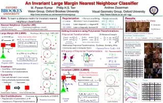
An Invariant Large Margin Nearest Neighbour Classifier. Vision Group, Oxford Brookes University. Visual Geometry Group, Oxford University. http://cms.brookes.ac.uk/research/visiongroup. http://www.robots.ox.ac.uk/~vgg.

E N D
An Invariant Large Margin Nearest Neighbour Classifier Vision Group, Oxford Brookes University Visual Geometry Group, Oxford University http://cms.brookes.ac.uk/research/visiongroup http://www.robots.ox.ac.uk/~vgg Aim:To learn a distance metric for invariant nearest neighbour classification Results Regularization • Prevent overfitting • Retain convexity Matching Faces from TV Video min ∑ iM(i,i) Minimize L2 norm of parameter L • L2-LMNN M(i,j) = 0, i ≠ j Learn diagonal L diagonal M • D-LMNN Nearest Neighbour Classifier (NN) 11 characters 24,244 faces min ∑ i,j |M(i,j)|, i ≠ j • Find nearest neighbours, classify • Typically, Euclidean distance used • Multiple classes • Labelled training data • DD-LMNN Learn a diagonally dominant M Adding Invariance using Polynomial Transformations Large Margin NN (LMNN) Weinberger, Blitzer, Saul - NIPS 2005 Invariance to changes in position of features Polynomial Transformations 2D Rotation Example Euclidean Transformation x Lx Same class points closer 1 cos θ -sin θ -(θ-θ3/6) 1-θ2/2 a a a b -a/2 b/6 -5o ≤ ≤ 5o -3 ≤ tx ≤ 3 pixels -3 ≤ ty ≤ 3 pixels = θ min ∑ ij dij = (xi-xj)TLTL(xi-xj) sin θ b b a -b/2 -a/6 b cos θ (θ-θ3/6) 1-θ2/2 RDRD θ2 θ3 True Positives Univariate Transformation First Experiment (Exp1) X Taylor’s Series Approximation X min ∑ ij(xi-xj)TM(xi-xj) • Randomly permute data • Train/Val/Test - 30/30/40 • Suitable for NN xi xj • Multivariate Polynomial Transformations - Euclidean, Similarity, Affine M 0 (Positive Semidefinite) • Commonly used in Computer Vision • General Form: T(x,) = X Euclidean Distance Second Experiment (Exp2) Different class points away A Property of Polynomial Transformations dij SD - Representability • No random permutation • Train/Val/Test - 30/30/40 • Not so suitable for NN (xi-xk)TM(xi-xk)- (xi-xj)TM(xi-xj) 1 P 0 xk Dij ≥ 1 - eijk xi xj Lasserre, 2001 Mij Accuracy mij min ∑ ijkeijk, eijk ≥ 0 Semidefinite Program (SDP) P’ 0 2 (θ1 ,θ2) Learnt Distance Globally Optimum M (and L) Distance between Polynomial Trajectories SD - Representability of Segments Sum of Squares Of Polynomials Drawbacks -T ≤ ≤ T • Overfitting - O(D2) parameters Invariant LMNN (ILMNN) x Lx • No invariance to transformations dij Minimize Max Distance of same class trajectories Current Fix Euclidean Distance xi xj • Use rank deficient L (non-convex) Non-convex Euclidean Distance Mij • Add synthetically transformed data Approximation: ijdij ij = Precision-Recall Timings 1 mij • Inefficient • Inaccurate min ∑ ij ijdij Dik(1,2) E X P 1 Euclidean Distance Maximize Min Distance of different class trajectories xk 2 Transformation Trajectory Finite Transformed Data Learnt Distance Dik(1,2) - ijdij ≥ 1 - eijk E X P 2 Our Contributions Overcome above drawbacks of LMNN Pijk 0 (SD-representability) • Regularization of parameters L or M Convex SDP Preserve Convexity min ∑ ijkeijk, eijk ≥ 0 • Invariance to Polynomial Transformations Learnt Distance