Download
1 / 15
150 likes | 352 Views
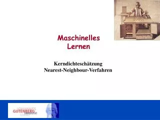
Maschinelles Lernen. Kerndichteschätzung Nearest-Neighbour-Verfahren. Kerndichteschätzung.

E N D
Maschinelles Lernen KerndichteschätzungNearest-Neighbour-Verfahren
Kerndichteschätzung Idee: Bei gegebenen Daten D={x1,…,xN}Verwende die Datenpunkte in der Umgebung eines Punktes x zur Schätzung von p(x) (bzw. zur Schätzung von p(x|ω), falls verschiedene Klassen ω gelernt werden sollen). Setze und Dann ist eine Approximation von p(x). Fragen: Wie muss V gewählt werden? Wie groß muss k sein? Ist eine Dichte?
Kerndichteschätzung Wahre Dichte
Parzen Windows, Nearest Neighbours Asymptotik für wachsende Zahl von Datenpunkten N: Notwendige Kriterien für : Zwei Möglichkeiten für die praktische Wahl von kN,VN bei gegebener Zahl von Datenpunkten N: 1. Wähle VN, z.B. VN = N-0.5. Dann erwartet man im Mittel kN = N0.5 Punkte pro Volumeneinheit, und kN/N = N-0.5. (Parzen Window Methode) 2. Wähle kN, z.B. kN = N0.5. Vergrößere das Volumen so lange, bis es kN Punkte enthält. Man erwartet im Mittel VN = N-0.5 Punkte pro Volumeneinheit, und kN/N = N-0.5. (Nearest Neighbour Methode)
Parzen Windows, Nearest Neighbours 1. Wähle VN, z.B. VN = N-0.5. Dann erwartet man im Mittel kN = N0.5 Punkte pro Volumeneinheit, und kN/N = N-0.5. (Parzen Window Methode) Parzen Windows Nearest Neighbours 2. Wähle kN, z.B. kN = N0.5. Vergrößere das Volumen so lange, bis es kN Punkte enthält. Man erwartet im Mittel VN = N-0.5 Punkte pro Volumeneinheit, und kN/N = N-0.5. (k-Nearest Neighbour Methode, kNN) Aus: Duda, Hart, Stork. Pattern Recognition
Kerndichteschätzung Die Gestalt des Volumens ist noch nicht festgelegt. Wählt man jenes als einen Hyperkubus mit Zentrum x und Kantenlänge hN, so hat man: und mit schreibt sich daraus folgt (bei p-dimensionalen Daten)
Kerndichteschätzung Verallgemeinerung: Ist die Funktion ρ selbst eine Dichte, so auch (Beweis: Übung) Definiere für beliebige Kerndichteρ und „Fensterbreite“ h :
Kerndichteschätzung Dichteschätzungen für N=5 Datenpunkte und verschiedene Intervallbreiten. Dichte = Standardnormalverteilung Aus: Duda, Hart, Stork. Pattern Recognition
Kerndichteschätzung Gebräuchliche Kerndichten sind: Gauß Kernel Epanechnikov Kernel Tri-cube Kernel
Kerndichteschätzung Klassifikation: Schätze p(x|ω1) und p(x|ω2) und fälle (evtl. nach zusätzlichen a priori-Annahmen über p(ωk) ) danach eine ML bzw. eine MAP-Entscheidung. Aus: Duda, Hart, Stork. Pattern Recognition
Kerndichteschätzung Die Fensterbreite h bestimmt, wie stark sich die geschätzte Dichte den Daten anpasst. Wie immer ist auf einen Kompromiss zwischen Bias und Varianz zu achten. Eine zu kleine Fensterbreite produziert eine Überanpassung an die Daten (“overfitting”). eine zu große Fensterbreite übergewichtet die initial angenommene Dichte (“underfitting”). Beides führt zu schlechten Verallgemeinerungseigen-schaften der Modelle.
Exkurs: kNN/Parzen Windows und Regression The idea is to replace the k-nearest neighbours average by a more robust estimate. Generalize the regression function by weighting the contribution of each yj to the regression function at the point x: Narada-Watson weighted average Here, K(x,z) is the so-called regression kernel which determines the influence of the point zєX on the regression function at x. In order to obtain a sensible regression function, a point z close to x should have a higher impact than a point further away, so the kernel function K(x,z) needs to be bell-shaped around x (as a function of z). Exkurs: kNN Regression Note that the result of the choice is k-nearest neighbours averaging. Usually, the kernel is chosen to be translation invariant, so it can be written as
Exkurs: kNN Regression Like the parameter k for nearest neighbours, the parameter λ determines the tradeoff between bias and variance in the prediction error and need to be chosen carefully (the sample data is given by the black points) : λ small λ medium λ large
Exkurs: kNN Regression The result of a weighted regression is a smooth function. However, the bias of such a weighted regression function at the boundaries of the domain X is rather (if f is non-constant at the boundaries). An idea to remove this bias is to combine linear regression with a kernel weighting scheme: For each point xєX, solve the weighted linear regression with Kλone of the mentioned kernel functions. For every x, this yields a local regression function fx(t)=αx+βxt. The function fx is then evaluated only at the point t=x in order to obtain the (global) regression function
Exkurs: kNN Regression Taken from: Tibshirani et al. „Elements of Statistical Learning“