Poles and Zeros

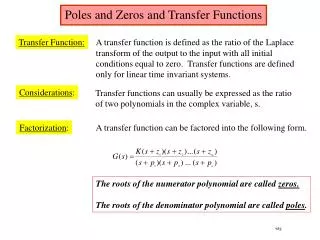
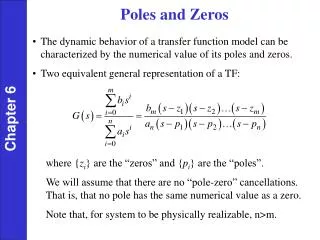
1. Poles and Zeros • The dynamic behavior of a transfer function model can be characterized by the numerical value of its poles and zeros. • Two equivalent general representation of a TF: Chapter 6 where {zi} are the “zeros” and {pi} are the “poles”. We will assume that there are no “pole-zero” cancellations. That is, that no pole has the same numerical value as a zero. Note that, for system to be physically realizable, n>m.

2. Example: 4 poles (denominator is 4th order polynomial) & 0 zero (numerator is a const)

3. Chapter 6

4. Effects of Poles on System Response

5. Example of Integrating Element pure integrator (ramp) for step change in qi

6. Cause of Zeros – Input Dynamics

7. Some Facts about Zeros • Zeros do not affects the number and locations of the poles, unless there is an exact cancellation of a pole by a zero. • The zeros exert a profound effect on the coefficients of the response modes.

8. Example of 2nd-Order Overdamped System with One (1) Zero

9. Chapter 6

10. Step Response of 2nd-Order OverdampedSystem without Zeros

11. Further Analysis of Inverse Response

12. Chapter 6

13. Common Properties of Overshoot and Inverse Responses

14. Another Example

15. Time Delays Time delays occur due to: • Fluid flow in a pipe • Transport of solid material (e.g., conveyor belt) • Chemical analysis • Sampling line delay • Time required to do the analysis (e.g., on-line gas chromatograph) Chapter 6 Mathematical description: A time delay, , between an input u and an output y results in the following expression:

16. Chapter 6

17. Implication of Time Delay The presence of time delay in a process means that we cannot factor the transfer function in terms of simple poles and zeros!

18. Polynomial Approximation of Time Delays

19. Chapter 6

20. Approximation of nth-Order Systems

21. Approximation of Higher-Order Transfer Functions In this section, we present a general approach for approximating high-order transfer function models with lower-order models that have similar dynamic and steady-state characteristics. Previously we showed that the transfer function for a time delay can be expressed as a Taylor series expansion. For small values of s, Chapter 6 An alternative first-order approximation is

22. Skogestad’s“Half Rule” • Largest neglected time constant • One half of its value is added to the existing time delay (if any) . • The other half is added to the smallest retained time constant. • Time constants that are smaller than those in item 1. • Use (B) • RHP zeros. • Use (A) Chapter 6

23. Example 6.4 Consider a transfer function: Derive an approximate first-order-plus-time-delay (FOPDT) model, Chapter 6 • using two methods: • The Taylor series expansions (A) and (B). • Skogestad’s half rule Compare the normalized responses of G(s) and the approximate models for a unit step input.

24. Solution • The dominant time constant (5) is retained. Applying • the approximations in (A) and (B) gives: and Chapter 6 Substitution into G(s) gives the Taylor series approximation,

25. (b) To use Skogestad’s method, we note that the largest neglected time constant in G(s) has a value of three. • According to “half rule” (Rule 1), half of this value is added to the next largest time constant to generate a new time constant • Rule 1: The other half provides a new time delay of 0.5(3) = 1.5. • The approximation of the RHP zero in Rule 3 provides an additional time delay of 0.1. • Approximating the smallest time constant of 0.5 in G(s) by Rule 2 produces an additional time delay of 0.5. • Thus the total time delay is, • Therefore Chapter 6

26. Chapter 6

27. Example

28. Part (a)

29. Part (b)