LECTURE 09: BAYESIAN ESTIMATION (Cont.)
LECTURE 09: BAYESIAN ESTIMATION (Cont.). • Objectives: Bayesian Estimation Example Resources: D.H.S.: Chapter 3 (Part 2) J.O.S.: Bayesian Parameter Estimation A.K.: The Holy Trinity A.E.: Bayesian Methods J.H.: Euro Coin. Sufficient Statistics.

LECTURE 09: BAYESIAN ESTIMATION (Cont.)
E N D
Presentation Transcript
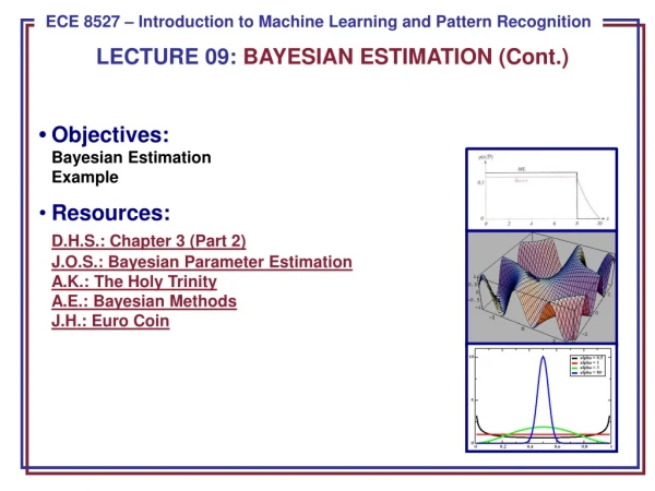
LECTURE 09: BAYESIAN ESTIMATION (Cont.) • Objectives:Bayesian EstimationExample • Resources: • D.H.S.: Chapter 3 (Part 2)J.O.S.: Bayesian Parameter EstimationA.K.: The Holy TrinityA.E.: Bayesian MethodsJ.H.: Euro Coin
Sufficient Statistics • Direct computation of p(D|θ)and p(θ|D)for large data sets is challenging(e.g. neural networks) • We need a parametric form for p(x|θ)(e.g., Gaussian) • Gaussian case: computation of the sample mean and covariance, which was straightforward, contained all the information relevant to estimating the unknown population mean and covariance. • This property exists for other distributions. • A sufficient statistic is a function s of the samples D that contains all the information relevant to a parameter, θ. • A statistic, s, is said to be sufficient for θif p(D|s,θ)is independent of θ:
The Factorization Theorem • Theorem: A statistic, s, is sufficient for θ, if and only if p(D|θ)can be written as: . • There are many ways to formulate sufficient statistics(e.g., define a vector of the samples themselves). • Useful only when the function g() and the sufficient statistic are simple(e.g., sample mean calculation). • The factoring of p(D|θ)is not unique: • Define a kernel density invariant to scaling: • Significance: most practical applications of parameter estimation involve simple sufficient statistics and simple kernel densities.
Gaussian Distributions • This isolates the θdependence in the first term, and hence, the sample mean is a sufficient statistic using the Factorization Theorem. • The kernel is:
The Exponential Family • This can be generalized: and: • Examples:
Probability of Error • Feature vectors typically have dimensions greater than 50. • Classification accuracy depends upon the dimensionality and the amount of training data. • Consider the case of two classes multivariate normal with the same covariance: where:and: • If the features are independent then: , • and
Dimensionality and Training Data Size • The most useful features are the ones for which the difference between the means is large relative to the standard deviation . • Too many features can lead to a decrease in performance. • Fusing of different types of information, referred to as feature fusion, is a good application for Principal Components Analysis (PCA). • Increasing the feature vector dimension can significantly increase the memory (e.g., the number of elements in the covariance matrix grows as the square of the dimension of the feature vector) and computational complexity. • Good rule of thumb: 10 independent data samples for every parameter to be estimated. • For practical systems, such as speech recognition, even this simple rule can result in a need for vast amounts of data.
Computational Complexity • “Big Oh” notation used to describe complexity:if f(x) = 2+3x+4x2, f(x) has computational complexity O(x2) • Recall: • Watch those constants of proportionality (e.g., O(nd2)). • If the number of data samples is inadequate, we can experience overfitting (which implies poor generalization). • Hence, later in the course, we will study ways to control generalization and to smooth estimates of key parameters such as the mean and covariance (see textbook).
Overfitting • It is common that the number of available samples is inadequate to train a complex classifier. Alternatives: • Reduce the number of parameters(e.g., assume diagonal covariances) • Assume all classes have the same covariance (“pooled covariance”) • Better estimate of covariance (e.g., use Bayesian parameter estimate) • Pseudo-Bayesian estimate: • Regularized discriminant analysis (shrinkage):
Component Analysis • Previously introduced as a “whitening transformation”. • Component analysis is a technique that combines features to reduce the dimension of the feature space. • Linear combinations are simple to compute and tractable. • Project a high dimensional space onto a lower dimensional space. • Three classical approaches for finding the optimal transformation: • Principal Components Analysis (PCA): projection that best represents the data in a least-square sense. • Multiple Discriminant Analysis (MDA): projection that best separates the data in a least-squares sense. • Independent Component Analysis (IDA): projection that minimizes the mutual information of the components.
Principal Component Analysis • Consider representing a set of n d-dimensional samples x1,…,xnby a single vector, x0. • Define a squared-error criterion: • It is easy to show that the solution to this problem is given by: • The sample mean is a zero-dimensional representation of the data set. • Consider a one-dimensional solution in which we project the data into a line running through the sample mean: • where e is a unit vector in the direction of this line, and a is a scalar representing the distance of any point from the mean. • We can write the squared-error criterion as:
Minimizing Squared Error • Note that: (the norm of the unit vector is 1) • Differentiate with respect to ak and obtain: • The geometric interpretation is the we obtain a least-squares solution by projecting the vector, x, onto a line in the direction of e that passes through the sample mean. • But what is the best direction for e?
Scatter Matrix • Define a scatter matrix, S: • This should look familiar, it is (n-1) times the sample covariance matrix. • If we substitute our solution for ak into our expression for the squared error:
Minimization Using Lagrange Multipliers • The vector, e, that minimizes J1 also maximizes . • Use Lagrange multipliers to maximize subject to the constraint . • Let be the undetermined multiplier, and differentiate: • with respect to e, to obtain: • Set to zero and solve: • It follows to maximize we want to select an eigenvector corresponding to the largest eigenvalue of the scatter matrix. • In other words, the best one-dimensional projection of the data (in the least mean-squared error sense) is the projection of the data onto a line through the sample mean in the direction of the eigenvector of the scatter matrix having the largest eigenvalue (hence the name Principal Component). • For the Gaussian case, the eigenvectors are the principal axes of the hyperellipsoidally shaped support region! • Let’s work some examples (class-independent and class-dependent PCA).
Summary • Introduction of Bayesian parameter estimation. • The role of the class-conditional distribution in a Bayesian estimate. • Estimation of the posterior and probability density function assuming the only unknown parameter is the mean, and the conditional density of the “features” given the mean, p(x|θ), can be modeled as a Gaussian distribution. • Bayesian estimates of the mean for the multivariate Gaussian case. • General theory for Bayesian estimation. • Comparison to maximum likelihood estimates. • Recursive Bayesian incremental learning. • Noninformative priors. • Sufficient statistics • Kernel density.

