Download
1 / 1
10 likes | 118 Views
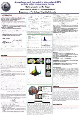
Anxiety-related response. Instruction-related response. Speech topic instruction. “No speech” instruction. Speech preparation. Fixation baseline. Fixation baseline. Task design: Anxiogenic task. A. C. 1. 1. 2. 3. 2. B. 3.

E N D
Anxiety-related response Instruction-related response Speech topic instruction “No speech” instruction Speech preparation Fixation baseline Fixation baseline Task design: Anxiogenic task A C 1 1 2 3 2 B 3 A novel approach to modeling state-related fMRI activity using change-point theory Martin Lindquist and Tor Wager Department of Statistics, Columbia University Department of Psychology, Columbia University INTRODUCTION • HEWMA: A hierarchical extension of EWMA • Interest in fMRI in population inference • Approach: EWMA for each subject; mixed-effects (hierarchical) test of significance across subjects at 2nd level • Suppose the EWMA statistic at time t for subject i, which we denote Zti, is defined as in Eq. 1. The HEWMA statistic is a weighted average of the individual EWMA statistics, with the weights inversely proportional to the total variance for each subject, i.e. • [3] • where . Here i* is the variance from the single subject EWMA analysis and b* is the between subject variance, known up to a scaling parameter . • Estimate using a restricted maximum likelihood (ReML) approach • Iterative estimation of Zpop and its variance components. • The final step in the HEWMA framework is performing a Monte Carlo simulation to get corrected p-values, except here we use Zpop and its covariance matrix in the simulation. • Goal: To develop and apply a hybrid hypothesis- and data-driven analysis for modeling sustained psychological states with uncertain onset time and duration; e.g., experienced emotion, learning, insight. • Need to balance inferential power of hypothesis-driven approaches (e.g. GLM) with flexibility of data-driven methods (e.g. ICA). • Our approach: Uses ideas from statistical control theory • Population inference on whether and when a timeseries changes from a baseline state • Handles uncertain onset times and durations • Simulations: false-positive rate (FPR) control and power • Application: fMRI study (n = 25) of state anxiety. • Toolbox: Matlab implementation freely available • http://www.columbia.edu/cu/psychology/tor/ Figure 2. (A-B) Simulated power and false positive rates for HEWMA with varying smoothness parameter, and fixed baseline length of 60 TRs. (C-D) Same plots with fixed lambda and varying baseline length. • Estimating Change points (CPs) • If a systematic deviation from baseline is detected, we estimate the time of change and recovery time (if any). • Zero-crossing method: use the last time point at which the process crosses 0 before becoming significant. Run duration: number of contiguous activated time points • MLE method: maximum likelihood estimates of • Gaussian mixture model method: 2-state (control and activated); classify time points in one of the two states. Estimate duration of activated runs as above. • Clustering into regions • A natural unit of analysis is a multi-voxel region whose voxels show similar properties We first obtain a Change Point Map (CPM) and Activation Duration Map over all significantly activated voxels • K-means clustering in 2-D (CP and duration) space. • Number of classes chosen based on histogram (Fig. 4). • Contiguous voxels of same class are “regions” Figure 1. A schematic overview of the model of true activation (boxcar) and the EWMA statistic zt (black line). Control limits for EWMA statistic deviations can be calculated as cVar(zt), where c is a critical t-value corresponding to the desired false positive-rate. Figure 3. (A) HEWMA group activation, Zpop, and the estimated CP (green line). (B) Results of Monte Carlo simulations for finding corrected p-values. Black line: observed max T; distribution: null hypothesis max T. (C) Case weights calculated according to Eq. (3). (D) The time courses for the 25 subjects • Simulations • Assess the FPR and power for the HEWMA method (N = 20) • Vary (Sim 1: 0.1, 0.3, 0.5, 0.7 and 0.9) and duration of the baseline period (Sim 2: 20, 40, 60 or 80 time points) • Error models in EWMA estimation: white noise (WN), AR(1), AR(2) and ARMA(1,1). • N = 20 subjects, b = 0.33 * i, 5000 replications • FPR simulation: null hypothesis data with no activation was created using actual fMRI noise time courses. • Power simulation: As above, with active period of length 50 time points was added to the noise data, Cohen’s d of 0.5. • Experimental design • 24 participants were scanned in a 3T GE magnet. Participants were informed that they were to be given two minutes to prepare a seven-minute speech, and that the topic would be revealed to them during scanning. They were told that after the scanning session, they would deliver the speech to a panel of expert judges, though there was “a small chance” that they would be randomly selected not to give the speech. After the start of acquisition, participants viewed a fixation cross for 2 min (resting baseline). At the end of this period, participants viewed an instruction slide for 15 s that described the speech topic, which was to speak about “why you are a good friend.” The slide instructed participants to be sure to prepare enough for the entire 7 min period. After 2 min of silent preparation, another instruction screen appeared (a ‘relief’ instruction, 15 s duration) that informed participants that they would not have to give the speech. An additional 2 min period of resting baseline followed, which completed the functional run (Fig. 5). During a run, a series of 215 images were acquired (TR = 2s). METHODS Our method is a multi-subject extension of the exponentially weighted moving average (EWMA, Fig. 1) method used in change-point analysis. The analysis uses activity collected during a baseline period to estimate noise characteristics in the signal, and then make inferences on whether, when, and for how long subsequent activity deviates from the baseline level. We extend existing EWMA models for individual subjects (a single time series) so that they are applicable to fMRI data, and develop a group analysis using a hierarchical model, which we term HEWMA (Hierarchical EWMA). The HEWMA method can be used to analyze fMRI data voxel-wise throughout the brain, data from regions of interest, or temporal components extracted using ICA or similar methods. • Detecting Change points • No a priori assumptions about the nature of changes in the fMRI signal • activation or deactivation, short or prolonged activation duration. • EWMA is a search for activity differences across time, correcting for multiple dependent comparisons tested • EWMA • Given observations in time X=(x1,x2,…xn) • Two-state model: baseline (“in-control”) and activated (“out of control”). Assume data is distributed normally: N(0,) for baseline and N(1,) for activated. • 0 is estimated from prespecified baseline period • After baseline, process is “in control” up to some unknown time , the change point (CP), when the state changes to activated (see Fig. 1). • The exponentially weighted moving-average (EWMA) statistic, , is a temporally smoothed version of the data, which is defined as: • for [1] • where 01 is a constant smoothing parameter chosen by the analyst (small gives more smoothing), and the starting value z0 is set equal to the baseline estimate of 0. • To test whether the process has changed states at time t, we compute a test statistic for each time point following the baseline: • [2] Figure 4. A) Left: Regions with significant activations in HEWMA (corrected over time and FDR-corrected over space). Right: Regions color-coded according to K-means classification (7 classes). B) Histogram of number of voxels by CP and activation duration, color-coded by estimated class. C) Axial slices of regions shown in A. RESULTS Simulations of group data showed that false positive rates were adequately controlled for all noise models. The HEWMA analysis on the experimental data revealed task-related changes consistent with previous literature, including activations in dorsolateral and rostral medial prefrontal cortices, middle temporal gyrus, and occipital cortex (Figs. 4 and 5). Deactivations were found in ventral striatum and ventral anterior insula. K-means classification of voxels by activation onset time and duration revealed distinct patterns of responses to the task (color-coded by class in Fig. 4). Time courses for two patterns of responses are shown in Fig. 5, including a medial prefrontal region showing sustained activity throughout the anxiogenic task and an occipital region showing transient responses to the instruction periods (when visual stimuli were presented). • where Var(zt) is the (co-)variance of the EWMA statistic at time t. • Theoretical results for Var(zt) for a variety of noise models is provided in Lindquist and Wager (2006). • Under the null hypothesis T follows a t-distribution. • Family-wise error rate control across the time series is provided using Monte Carlo integration • Generate null hypothesis data with covariance given by Var(zt) • Save the maximum absolute T-value obtained across the time series • Compare observed T values against distribution of maxima REFERENCES Figure 5. The brain surface is shown in lateral oblique and axial views. Significant voxels are colored according to significance. Increases are shown in red-yellow, and decreases are shown in light-dark blue. (A) Time course from a region showing sustained activity in rostral medial PFC (single representative voxel). The baseline period is indicated by the shaded gray box, and the HEWMA-statistic is shown by the thick black line (+/- one standard error across participants, shown by gray shading). The control limits are shown by dashed lines. (B) A similar plot showing transient responses to presentation of task instructions in visual cortex. Lindquist & Wager. “Application of change-point theory to modeling state-related activity in fMRI”. In Pat Cohen (Ed), Applied Data Analytic Techniques for "Turning Points Research. In press, 2006.