Download
1 / 39
390 likes | 470 Views
Explore gene recognition techniques such as Generalized HMMs and Pair HMMs for alignments to understand gene structure, transcription, splicing, and translation. Learn about Twinscan algorithm and approaches for gene finding. Discover the biology of splicing and sequence identity in orthologous genes.

E N D
Gene Recognition Credits for slides: Marina Alexandersson Lior Pachter Serge Saxonov
Reading • GENSCAN • SLAM • Twinscan Optional: Chris Burge’s Thesis Lecture 13, Thursday May 15, 2003
Gene expression DNA transcription RNA translation Protein CCTGAGCCAACTATTGATGAA CCUGAGCCAACUAUUGAUGAA PEPTIDE Lecture 13, Thursday May 15, 2003
Gene structure intron1 intron2 exon2 exon3 exon1 transcription splicing translation exon = coding intron = non-coding Lecture 13, Thursday May 15, 2003
Exon 3 Exon 1 Exon 2 Intron 1 Intron 2 5’ 3’ Stop codon TAG/TGA/TAA Start codon ATG Finding genes Splice sites Lecture 13, Thursday May 15, 2003
Approaches to gene finding • Homology • BLAST, Procrustes. • Ab initio • Genscan, Genie, GeneID. • Hybrids • GenomeScan, GenieEST, Twinscan, SGP, ROSETTA, CEM, TBLASTX, SLAM. Lecture 13, Thursday May 15, 2003
intron exon exon intron intergene exon intergene HMMs for gene finding GTCAGAGTAGCAAAGTAGACACTCCAGTAACGC Lecture 13, Thursday May 15, 2003
T A A T A T G T C C A C G G G T A T T G A G C A T T G T A C A C G G G G T A T T G A G C A T G T A A T G A A Exon1 Exon2 Exon3 GHMM for gene finding Lecture 13, Thursday May 15, 2003
Observed duration times Lecture 13, Thursday May 15, 2003
Biology of Splicing (http://genes.mit.edu/chris/) Lecture 13, Thursday May 15, 2003
Consensus splice sites Donor: 7.9 bits Acceptor: 9.4 bits (Stephens & Schneider, 1996) (http://www-lmmb.ncifcrf.gov/~toms/sequencelogo.html) Lecture 13, Thursday May 15, 2003
Splice Site Models • WMM: weight matrix model = PSSM (Staden 1984) • WAM: weight array model = 1st order Markov (Zhang & Marr 1993) • MDD: maximal dependence decomposition (Burge & Karlin 1997) decision-tree like algorithm to take significant pairwise dependencies into account Lecture 13, Thursday May 15, 2003
Donor site 5’ 3’ Position % Splice site detection Lecture 13, Thursday May 15, 2003
atg caggtg ggtgag cagatg ggtgag cagttg ggtgag caggcc ggtgag tga
Coding potential Amino Acid SLC DNA codons Isoleucine I ATT, ATC, ATA Leucine L CTT, CTC, CTA, CTG, TTA, TTG Valine V GTT, GTC, GTA, GTG Phenylalanine F TTT, TTC Methionine M ATG Cysteine C TGT, TGC Alanine A GCT, GCC, GCA, GCG Glycine G GGT, GGC, GGA, GGG Proline P CCT, CCC, CCA, CCG Threonine T ACT, ACC, ACA, ACG Serine S TCT, TCC, TCA, TCG, AGT, AGC Tyrosine Y TAT, TAC Tryptophan W TGG Glutamine Q CAA, CAG Asparagine N AAT, AAC Histidine H CAT, CAC Glutamic acid E GAA, GAG Aspartic acid D GAT, GAC Lysine K AAA, AAG Arginine R CGT, CGC, CGA, CGG, AGA, AGG Stop codons Stop TAA, TAG, TGA Lecture 13, Thursday May 15, 2003
Comparison of 1196 orthologous genes(Makalowski et al., 1996) • Sequence identity: • exons: 84.6% • protein: 85.4% • introns: 35% • 5’ UTRs: 67% • 3’ UTRs: 69% • 27 proteins were 100% identical. Lecture 13, Thursday May 15, 2003
Human Mouse Human-mouse homology Lecture 13, Thursday May 15, 2003
Not always: HoxA human-mouse Lecture 13, Thursday May 15, 2003
50 . : . : . : . : . : 247 GGTGAGGTCGAGGACCCTGCA CGGAGCTGTATGGAGGGCA AGAGC |: || ||||: |||| --:|| ||| |::| |||---|||| 368 GAGTCGGGGGAGGGGGCTGCTGTTGGCTCTGGACAGCTTGCATTGAGAGG 100 . : . : . : . : . : 292 TTC CTACAGAAAAGTCCCAGCAAGGAGCCACACTTCACTG |||----------|| | |::| |: ||||::|:||:-|| ||:| | 418 TTCTGGCTACGCTCTCCCTTAGGGACTGAGCAGAGGGCT CAGGTCGCGG 150 . : . : . : . : . : 332 ATGTCGAGGGGAAGACATCATTCGGGATGTCAGTG ---------------||||||||||||||||||||||:|||||||||||| 467 TGGGAGATGAGGCCAATGTCGAGGGGAAGACATCATTTGGGATGTCAGTG 200 . : . : . : . : . : 367 TTCAACCTCAGCAATGCCATCATGGGCAGCGGCATCCTGGGACTCGCCTA |||||:||||||||:||||||||||||||:|| ||:|||||:|||||||| 517 TTCAATCTCAGCAACGCCATCATGGGCAGTGGAATTCTGGGGCTCGCCTA Alignment Lecture 13, Thursday May 15, 2003
Twinscan • Twinscan is an augmented version of the Gencscan HMM. I E transitions duration emissions ACUAUACAGACAUAUAUCAU Lecture 13, Thursday May 15, 2003
Twinscan Algorithm • Align the two sequences (eg. from human and mouse) • Mark each human base as gap ( - ), mismatch ( : ), match ( | ) New “alphabet”: 4 x 3 = 12 letters = { A-, A:, A|, C-, C:, C|, G-, G:, G|, U-, U:, U| } Lecture 13, Thursday May 15, 2003
Twinscan Algorithm (cont’d) • Run Viterbi using emissions ek(b) where b { A-, A:, A|, …, T| } Note: Emission distributions ek(b) estimated from real genes from human/mouse eI(x|) < eE(x|): matches favored in exons eI(x-) > eE(x-): gaps (and mismatches) favored in introns Lecture 13, Thursday May 15, 2003
Example Human: ACGGCGACUGUGCACGU Mouse: ACUGUGAC GUGCACUU Align: ||:|:|||-||||||:| Input to Twinscan HMM: A| C| G: G| C: G| A| C| U- G| U| G| C| A| C| G: U| Recall, eE(A|) > eI(A|) eE(A-) < eI(A-) Likely exon Lecture 13, Thursday May 15, 2003
HMMs for simultaneous alignment and gene finding: Generalized Pair HMMs
A Pair HMM for alignments 1 - 2 M P(xi, yj) 1- - 2 1- - 2 I P(xi) J P(yj) BEGIN I M J END Lecture 13, Thursday May 15, 2003
Cross-species gene finding Exon3 Exon1 Exon2 Intron1 Intron2 5’ 3’ CNS CNS CNS [human] [mouse] Exon = coding Intron = non-coding CNS = conserved non-coding Lecture 13, Thursday May 15, 2003
Generalized Pair HMMs Lecture 13, Thursday May 15, 2003
Ingredients in exon scores • Splice site detection (VLMM) • Length distribution (generalized) • Coding potential (codon freq. tables) • GC-stratification Lecture 13, Thursday May 15, 2003
Exon GPHMM 1.Choose exon lengths (d,e). 2.Generate alignment of length d+e. e d Lecture 13, Thursday May 15, 2003
The SLAM hidden Markov model Lecture 13, Thursday May 15, 2003
Example: HoxA2 and HoxA3 TBLASTX SLAM SLAM CNS SGP-2 VISTA Twinscan RefSeq Genscan Lecture 13, Thursday May 15, 2003
length seq1 no. states length seq2 max duration Computational complexity Lecture 13, Thursday May 15, 2003
Approximate alignment Reduces TU -factor to hT Lecture 13, Thursday May 15, 2003
Measuring Performance • Definition: • Sensitivity (SN): (# correctly predicted)/(# true) • Specificity (SP): (# correctly predicted)/(# total predicted) Lecture 13, Thursday May 15, 2003
Measuring Performance Lecture 13, Thursday May 15, 2003