Download
1 / 21
210 likes | 415 Views
Chapter V Frictionless Duct Flow with Heat Transfer.

E N D
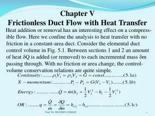
Chapter VFrictionless Duct Flow with Heat Transfer Heat addition or removal has an interesting effect on a compress- ible flow. Here we confine the analysis to heat transfer with no friction in a constant-area duct. Consider the elemental duct control volume in Fig. 5.1. Between sections 1 and 2 an amount of heat δQ is added (or removed) to each incremental mass δm passing through. With no friction or area change, the control-volume conservation relations are quite simple. Prof. Dr. MOHSEN OSMAN
Fig. (5.1) Elemental control volume for frictionless flow in a constant-area duct with heat transfer. The length of the element is determined in this simplified theory. Control volume \ No friction A2 = A1 \ V1 , P1 , T1 , To1 V2 , P2 , T2 , To2 The heat transfer results in a change in stagnation enthalpy of the flow. We shall not specify exactly how the heat is transferred; combustion, nuclear reaction, evaporation, condensation, or wall heat exchange, but simply that it happened in amount q between 1 and 2. We remark, however, that wall heat exchange is not a good candidate for the theory because wall convection is inevitably coupled with wall friction, which we neglected. To complete the analysis we use the perfect gas and Mach-number relations. Prof. Dr. MOHSEN OSMAN
For a given heat transfer or, equivalently, a given change can besolved algebraically for the property ratios between inlet and outlet. Notethat because the heat transferallows the entropy either to increase or decrease, thesecond law imposes no restrictions on these solutions Fig.(5.2) Effect of Heat Transfer Mach number. Prof. Dr. MOHSEN OSMAN
Before writing down these property ratio functions, we illustrate the effect of heat transfer in Fig.(5.2), which shows To and T versus Mach number in the duct. Heating increases To , and cooling decreases it. The maximum possible To occurs at M = 1.0, and we see that heating, whether the inlet is subsonic or supersonic, drives the duct Mach number toward unity. This is analogus to the effect of friction in the previous chapter. The temperature of a perfect gas (T) increases from M = 0.0 up to and then decreases. Thus there is a peculiar–or at least unexpected–region where heating (increasing To ) actually decreases the gas temperature, the difference being reflected in a large increase of the gas kinetic energy. Prof. Dr. MOHSEN OSMAN
For γ = 1.4, this peculiar area lies between M = 0.845 and 1.0 (interesting but not very useful information). The complete list of effects of simple To change on duct-flow properties is as follows: † Increases up to M = 1/√γ and decreases thereafter. ‡ Decreases up to M = 1/√γ and increases thereafter. Prof. Dr. MOHSEN OSMAN
Probably the most significant item on this list is the stagnation pressure Po , which always decreases during heating whether the flow is subsonic or supersonic. Thus, heating does increases the Mach number of a flow but entails a loss in effective pressure recovery. Mach – Number Relations Equations (5.1) and (5.2) can be rearranged in terms of the Mach number and the results tabulated. For convenience we specify that the outlet section is sonic, M=1, with reference properties To*, T*, P*, ρ* , V*, and P*o . The inlet is assumed to be at arbitrary Mach number M. Eq(5.1) and (5.2) then take the following form: Prof. Dr. MOHSEN OSMAN
.. These formulas are all tabulated versus Mach number in table. The tables are very convenient if inlet properties M1, V1, etc., are given but are somewhat cumbersome if the given inform-ation centers on To1 and To2 . Let us illustrate with an example. Prof. Dr. MOHSEN OSMAN
Example 5.1 A fuel-air mixture, assumed thermodynamically equivalent to air with γ = 1.4, enters a duct combustion chamber at V1= 250 ft/s, P1 = 20 psia, and T1 = 530oR. The heat addition by combustion is 400 Btu per pound of mixture. Compute (a) the exit properties V2 , P2 , and T2 and (b) the total heat addition which would have caused a sonic exit flow. Solution (a)First convert the heat addition to aDuct Combustion Chamber change in To of the gas : V1=250 ft/s Po2 P1=20 psia P2 T1=530o.R V2 To1 , Po1 T2 , To2 Prof. Dr. MOHSEN OSMAN
We have enough information to compute M1 and To1 :Now use Eq.(5.3a) or interpolate into Table to find the inlet ratio corresponding to M1 = 0.222 , we get At the exit section we can now compute To2 = To1 + 1667 = 535 + 1667 = 2202oR Thus, we can compute the exit ratio Prof. Dr. MOHSEN OSMAN
From Eq.(5.3a) or interpolation into Table, we find that With inlet and exit Mach numbers known, we can tabulate the velocity, pressure, and temperature ratios as follows:Then the exit properties are given: Prof. Dr. MOHSEN OSMAN
(b) The maximum heat addition allowed without choking would drive the exit Mach number to unity. .. Prof. Dr. MOHSEN OSMAN
Choking Effects Due to Simple Heating Equation (5.3a) and Table indicate that the maximum possible stagnation temperature in simple heating corresponds to , or sonic exit Mach number. Thus, for given inlet conditions, only a certain maximum amount of heat can be added to the flow, for example, 488 Btu/lb in Example 5.1. For a subsonic inlet there is no theoretical limit on heat addition; the flow chokes more and more as we add more heat, with the inlet velocity approaching zero. For supersonic flow, even if M1 is infinite, there is a finite ratio for γ = 1.4. Thus, if heat added without limit to a supersonic flow, a normal-shock-wave adjustment is required to accommodate to the required property changes. . . Prof. Dr. MOHSEN OSMAN
In subsonic flow there is no theoretical limit to the amount of cooling allowed : the exit flow just becomes slower and slower, and the temperature approaches zero. In supersonic flow only a finite amount of cooling can be allowed before the exit flow approaches infinite Mach number, with and exit temperature equals to zero. There are very few practical applications for supersonic cooling. Example 5.2What happens to the inlet flow in Example 5.1, if the heat addition is increased to 600 Btu/lb and the inlet pressure and stagnation temperature are fixed ? What will the decrease in mass flux be ? Solution For q = 600 Btu/lb Prof. Dr. MOHSEN OSMAN
q = 600(25050) = 15,025,000 (ft.lbf)/slugthe flow will be choked at an exit stagnation temperature of … Hence and the flow will be choked down until this value corresponds to the proper subsonic Mach number. From Eq.(5.3a) or Table for It was specified that To1 and P1remain the same. The other inlet properties will change according to M1 : Prof. Dr. MOHSEN OSMAN
Finally, .From Example 5.1 The final result in mass flux is 9 percent less than the mass flux of 0.7912 slug/(ft2.s) in Example (5.1), due to the excess heat addition choking the flow. Prof. Dr. MOHSEN OSMAN
Proof of Mach Number Relations Given: Prof. Dr. MOHSEN OSMAN
.. Prof. Dr. MOHSEN OSMAN
Sincethen Prof. Dr. MOHSEN OSMAN
.. Relationship to the Normal-Shock WaveThe normal-shock-wave relations of chapter 3 actually lurk within the simple heating relations as a special case. From Table or Fig.(5.2) we see that for a given stagnation temper- ature less than T*o these are two flow satisfy the simple Prof. Dr. MOHSEN OSMAN
heating relations, one subsonic and the other supersonic. These two states have : (1) the same value of To , (2) the same mass flow per unit area, and (3) the same value of P+ρV2 . Therefore, these two states are exactly equivalent to the conditions on each side of normal-shock wave. The second law would again require that the upstream flow M1 be supersonic. To illustrate this point, take M1 = 3.0 and from Table read . Now, for the same value use Table or Eq.(5.3a) to compute The value of M2 is exactly what we read in the shock Table, as the downstream Mach number when M1 = 3.0. The pressure ratio for these two states is Prof. Dr. MOHSEN OSMAN
Which again is just what we read in Table, for M1=3. This illustration is meant only to show the physical background of the simple heating relations : it would be silly to make a practice of computing normal- shock wave in this manner. Prof. Dr. MOHSEN OSMAN