Download
1 / 36
380 likes | 677 Views
Organizing Principles for Learning in the Brain. Associative Learning: Hebb rule and variations, self-organizing maps Adaptive Hedonism: Brain seeks pleasure and avoids pain: conditioning and reinforcement learning Imitation: Brain specially set up to learn from other brains?

E N D
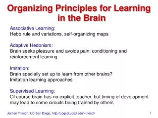
Organizing Principles for Learning in the Brain Associative Learning: Hebb rule and variations, self-organizing maps Adaptive Hedonism: Brain seeks pleasure and avoids pain: conditioning and reinforcement learning Imitation: Brain specially set up to learn from other brains? Imitation learning approaches Supervised Learning: Of course brain has no explicit teacher, but timing of development may lead to some circuits being trained by others
Classical Conditioning and Reinforcement Learning • Outline: • classical conditioning and its variations • Rescorla Wagner rule • instrumental conditioning • Markov decision processes • reinforcement learning Note: this presentation follows a chapter of “Theoretical Neuroscience” by Dayan&Abbott
Example of embodied models of reward based learning: Skinnerbots in Touretzky’s lab at CMU: http://www-2.cs.cmu.edu/~dst/Skinnerbots/index.html
Project Goals We are developing computational theories of operant conditioning. While classical (Pavlovian) conditioning has a well-developed theory, implemented in the Rescorla-Wagner model and its descendants (work by Sutton & Barto, Grossberg, Klopf, Gallistel, and others), there is at present no comprehensive theory of operant conditioning. Our work has four components: 1. Develop computationally explicit models of operant conditioning that reproduce classical animal learning experiments with rats, dogs, pigeons, etc. 2. Demonstrate the workability of these models by implementing them on mobile robots, which then become trainable robots (Skinnerbots). We originally used Amelia, a B21 robot manufactured by Real World Interface, as our implementation platform. We are moving to the Sony AIBO. 3. Map our computational theories onto neuroanatomical structures known to be involved in animal learning, such as the hippocampus, amygdala, and striatum. 4. Explore issues in human-robot interaction that arise when non-scientists try to train robots as if they were animals. also at: http://www-2.cs.cmu.edu/~dst/Skinnerbots/index.html
Pavlov’s classic finding: (classical conditioning) Initially, sight of food leads to dog salivating: food salivating unconditioned stimulus, US unconditioned response, UR (reward) Sound of bell consistently precedes food. Afterwards, bell leads to salivating: bell salivating conditioned stimulus, CS conditioned response, CR (expectation of reward) Classical Conditioning
Variations of Conditioning 1 Extinction: Stimulus (bell) repeatedly shown without reward (food): conditioned response (salivating) reduced. Partial reinforcement: Stimulus only sometimes preceding reward: conditioned response weaker than in classical case. Blocking (2 stimuli): First: stimulus S1 associated with reward: classical conditioning. Then: stimulus S1 and S2 shown together followed by reward: Association between S2 and reward not learned.
Variations of Conditioning 2 Inhibitory Conditioning (2 stimuli): Alternate 2 types of trials: 1. S1 followed by reward. 2. S1+S2 followed by absence of reward. Result: S2 becomes predictor of absence of reward. To show this use for example the following 2 methods: A. train animal to predict reward based on S2. Result: learning slowed B. train animal to predict reward based on S3, then show S2+S3. Result: conditioned response weaker than for S3 alone.
Variations of Conditioning 3 Overshadowing (2 stimuli): Repeatedly present S1+S2 followed by reward. Result: often, reward prediction shared unequally between stimuli. Example (made up): red light + high pitch beep precede pigeon food. Result: red light more effective in predicting the food than high pitch beep. Secondary Conditioning: S1 preceding reward (classical case). Then, S2 preceding S1. Result: S2 leads to prediction of reward. But: if S1 following S2 showed too often: extinction will occur
Summary of Conditioning Findings (incomplete, has been studied extensively for decades, many books on topic) figure taken from Dayan&Abbott
Modeling Conditioning The Rescorla Wagner rule (1972): Consider stimulus variable u representing presence (u=1) or absence (u=0) of stimulus. Correspondingly, reward variable r represents presence or absence of reward. The expected reward vis modeled as “stimulus x weight”: v = wu Learning is done by adjusting the weight to minimize error between predicted reward and actual reward.
Rescorla Wagner Rule Denote the prediction error by δ (delta): δ = r-v Learning rule: w := w + εδ u , whereεis a learning rate. Q: Why is this useful? A: This rule does stochastic gradient descent to minimize the expected squared error (r-v)2, w converges to <r>. R.W. rule is variant of the “delta rule” in neural networks. Note: in psychological terms the learning rate is measure of associability of stimulus with reward.
Rescorla Wagner Rule Example prediction error δ = r-v; learning rule: w := w + εδ u figure taken from Dayan&Abbott
Multiple Stimuli Essentially the same idea/learning rule: In case of multiple stimuli: v = w·u (predicted reward = dot product of stimulus vector and weight vector) Prediction error: δ = r-v Learning rule: w := w + εδu
In how far does Rescorla Wagner rule account for variants of classical conditioning? (prediction: v = w·u; error: δ = r-v; learning: w := w + εδu) figure taken from Dayan&Abbott
(prediction: v = w·u; error: δ = r-v; learning: w := w + εδu) Extinction, Partial Reinforcement: o.k., since w converges to <r> Blocking: during pre-training, w1 converges to r. During training v=w1u1+w2u2=r, hence δ=0 and w2 does not grow. Inhibitory Conditioning: on S1 only trials, w1 gets positive value. on S1+S2 trials, v=w1+w2 must converge to zero, hence w2 becoming negative. Overshadow: v=w1+w2 goes to r, but w1 and w2 may become different if there are different learning rates εifor them. Secondary Conditioning: R.-W.-rule predicts negative S2 weight! Rescorla Wagner rule qualitatively accounts for wide range of conditioning phenomena but not secondary conditioning.
Temporal Difference Learning Motivation: need to keep track of time within a trial Idea: (Sutton&Barto, 1990) Try to predict the total future reward expected from time t onward to the time T of end of trial. Assume time is in discrete steps. Predictedtotal future reward from time t (one stimulus case): Problem: how to adjust the weight? Would like to adjust w(τ) to make v(t) approximate the true total future reward R(t) (reward that is yet to come) but this is unknown since lying in future.
TD Learning cont’d. Solution: (Temporal Difference Learning Rule) , with temporal difference To see why this makes sense: We want v(t) to approximate left hand side but also: v(t+1) should approximate 2nd term of right hand side. Hence: or
TD Learning Rule Example ; reward and time course of reward correctly predicted! Note: temporal difference learning rule can also account for secondary conditioning (sorry, no example) figure taken from Dayan&Abbott
Dopamine and Reward Prediction (VTA= ventral tegmental area (midbrain)) VTA neurons fire for unex- pected reward: seem to re- present the prediction error δ figure taken from Dayan&Abbott
Instrumental Conditioning • So far: only concerned with prediction of reward. • Didn’t consider agent’s actions. Reward usually depends on what • you do! Skinnerboxes, etc. • Distinguish two scenarios: • Rewards follow actions immediately (Static Action Choice) • Example: n-armed bandit (slot machine) • B. Rewards may be delayed (Sequential Action Choice) • Example: playing chess • Goal: choose actions to maximize rewards
Static Action Choice Consider bee foraging: Bee can choose to fly to blue or yellow flowers, wants to maximize nectar volume. Bees learn to fly to “better” flower in single session (~40 flowers)
, where Simple model of bee foraging When bee chooses blue: reward ~p(rb) or yellow: reward ~p(ry) Assume model bee has stochastic policy: chooses to fly to blue or yellow flower with p(b) or p(y) respectively. A “convenient” assumption: p(b), p(y) follow softmax decision rule: Notes: p(b)+p(y)=1; mb, my are action values to be adjusted; β: inverse temperature: big β deterministic behavior
Exploration-Exploitation dilemma Why use softmax action selection? Idea: bee could also choose “better” action all the time. But: bee can’t be sure that better action is really better action. Bee needs to test and continuously verify which action leads to higher rewards. This is the famous exploration-exploitation dilemma of reinforcement learning: Need to explore to know what’s good. Need to exploit what you know is good to maximize reward. Generalization of softmax to many possible actions:
The Indirect Actor Question: how to adjust the action values ma ? Idea: have action values adapt to average reward for that action: mb = <rb> and my = <ry> This can be achieved with simple delta rule: mb mb + εδ , where δ = rb-mb This is indirect actor because action choice is mediated indirectly by expected amounts of rewards.
Indirect Actor Example figure taken from Dayan&Abbott
This leads to the following learning rule: where δab is the “Kronecker delta” and r is a parameter often chosen to be an estimate of the average reward per time. ¯ The Direct Actor Idea: choose action values directly to maximize expected reward Maximize this expected reward by stochastic gradient ascent: figure taken from Dayan&Abbott
Direct Actor Example again: nectar volumes reversed after first 100 visits figure taken from Dayan&Abbott
Sequential Action Choice So far: immediate reward after each action (n-armed bandit problem) Now:delayed rewards, can be in different states Example: Maze Task figure taken from Dayan&Abbott Amount of reward after decision at second intersection depends on action taken at first intersection.
Policy Iteration Big body of research on how to solve this and more complicated tasks, easily filling an entire course by itself. Here we just consider one example method:policy iteration. Assumption: state is fully observable (in contrast to only partially observable), i.e. the rat knows exactly where it is at any time. Idea: maintain and improve a stochastic policy, determining actions at each decision point (A,B,C) using action values and softmax decision. Two elements: critic: use temporal difference learning to predict future rewards from A,B,C if current policy is followed actor: maintain and improve the policy figure taken from Dayan&Abbott
Policy Iteration cont’d. How to formalize this idea? Introduce state variableu to describe whether rat is at A,B,C. Also introduce action value vectorm(u) describing the policy. (softmax rule assigns probability of action a based on action values) Immediate reward for taking action a in state u: ra(u) Expected future reward for starting in state u and following current policy: v(u) (state value). The rat’s estimate for this is denoted by w(u). Policy Evaluation (critic): estimate w(u) using temporal difference learning. Policy Improvement (actor): improve action values m(u)based on estimated state values. figure taken from Dayan&Abbott
Policy Evaluation Initially, assume all action values are 0, i.e. left/right equally likely everywhere. True value of each state can be found by inspection: v(B) = ½(5+0)=2.5; v(C) = ½(2+0)=1; v(A) = ½(v(B)+v(C))=1.75. These values can be learned with temporal difference learning rule: figure taken from Dayan&Abbott with where u’ is the state that results from taking action a in state u.
Policy Evaluation Example with figures taken from Dayan&Abbott
Policy Improvement How to adjust action values? where figures taken from Dayan&Abbott and p(a’;u) is the softmax probability of chosing action a’ in state u as determined by ma’(u). Example: consider starting out from random policy and assume state value estimates w(u) are accurate. Consider u=A, leads to rat will increase probability of going left in A for left turn for right turn
Policy Improvement Example figures taken from Dayan&Abbott
Some Extensions • -Introduction of a state vectoru • discounting of future rewards: put more • emphasis on rewards in the near future • than rewards that are far away. • Note: reinforcement learning is big subfield • of machine learning. There is a good • introductory textbook by Sutton and Barto.
Questions to discuss/think about • Even at one level of abstraction there are many different “Hebbian”, or Reinforcement learning rules; is it important which one you use? What is the right one? • The applications we discussed in Hebbian and Reinforcement learning considered networks passively receiving simple sensory input and learning to code it or behave “well”; how can we model learning through interaction with complex environments? Why might it be important to do so? • The problems we considered so far are very “low-level”, no hint of “complex behaviors” yet. How can we bridge this huge divide? How can we “scale up”? Why is it difficult?