Download

1 / 66
660 likes | 690 Views
Learn the theory, applications, and assumptions of Analysis of Variance (ANOVA) in various experimental designs. Understand the efficiency of different designs and techniques for dealing with wrongful data. Discover methods for checking ANOVA accuracy and interpreting results.

E N D
t-test |x1-x2| 2[(12+22)/(n1+n2)] t =
Multiple t-tests • Brundage v Lambert; Brundage v Croft; Brundage v Stephens; Lambert v Croft; Lambert v Stephens; Croft v Stephens. • Problems? • If all tests were done at 95% significance level, and one difference was significant, we have done 6 tests and would expect 1/20 to be significant, at random.
Analysis of Variance • Is an elegant and quicker way to calculate a pooled error term. • Analysis is simple in simple designs but can be complicated and lengthy in some designs (i.e. rectangular lattices). • In some experimental designs the ANOVA is the only method to estimate a pooled error term.
Analysis of Variance • It can provide an F-test to tests specific hypotheses. (i.e. to test general differences between different treatments). • Can be an invaluable initial contribution to interpretation of experiments.
Theory of Analysis of Variance ij(xij-x..)2 = ij[(xij-xi.) + (xi.-x..)]2 ij[(xij-xi.)2+2(xij-xi.)(xi.-x..)+(xi.-x..)2] ij(xij-x..)2 = ij(xij-xi.)2+ki(xi.-x..)2] ki(xi.-x..)2 = Between Treatment SS ij(xij-xi.)2 = Within Treatment SS
Theory of Analysis of Variance BTMS ~ 2n-1 df: WTMS ~ 2nk-n df 2n-1 df2nk-n df ~ F Dist n-1,nk-n df
Theory of Analysis of Variance [e2 + kt2]/e2 = 1, if kt2 = 0
Assumptions behind the ANOVA • Assumption of data being normally distributed. • Homogeneity of error variance. • Additivity of variance effects. • Data collected from a properly randomized experiment.
Analyses of CRB Designs Yij = + ti + eij
Analysis of Variance of CRB CF = [xij]2/jk
Analyses of RCB Designs Yij = + bi + tj + eij
Analysis of Variance of RCB CF = [xij]2/rt
Analyses of Latin Designs Yijk = + ri + cj + tk(ij) +eijk
Analysis of Variance of Latin CF = [xij]2/t2
Efficiency of Latin Squares cw CRB Design [MSr + MSc + (t-1)EMS]/(t+1)EMS If value response is 325, then latin square in will increase precision by 225% over CRB and CRD would have need 2.25 x 4 = 9 replicates to be as accurate.
Efficiency of Latin Squares cw RCB Design Row (RCB) = [MSr + (t-1)EMS]/(t+1)EMS Col(RCB) = [MSc + (t-1)EMS]/(t+1)EMS
+266% -19% ☺
-19% +226% ☺
Analyses of Lattice Squares Yijk = + ri + baj + tak +eijk
Efficiency of Lattice Design 100 x [Blk(adj)SS+Intra error SS]/k(k2-1)EMS 100 [11,382 + 14,533]/4(16)369 117% I II III IV V I II III IV V
Dealing with Wrongful Data • It is usually assumed that the data collected is correct!. • Why would data not be correct? • Mis-recording, mis-classification, transcription errors, errors in data entry. • Outliers.
Dealing with Wrongful Data • What things can help? • Keep detailed records, on each experimental unit. • Decide beforehand what values would arouse suspision.
Dealing with Wrongful Data • What do you do with suspicios data? • If correct, and it is discarded, then valuable information is lost. This will bias the results. • If wrong and included, will bias results and may have extreme consequences.
Checking ANOVA Accurucy • Coefficient of variation: [e/]x100. • CV=(√100.9/73.75)*100=13.6% • R2 value = {[TSS-ESS]/TSS}x100. • R2 = (1654/3654)*100 = 44.7%. • Compare the effect of blocking or sub-blocking (discussed later).
Marvelous Marvin father of the Groom Alaskan Wedding Feast
Expected Mean Squares • Dependant on whether factor effects are Fixed or Random. • Necessary to determine which F-tests are appropriate and which are not.
Setting Expected Mean Squares • The expected mean square for a source of variation (say X) contains. • the error term. • a term in 2x. (or S2x ) • a variance term for other selected interactions involving the factor X.
Coefficients for EMS Coefficient for error mean square is always 1 Coefficient of other expected mean squares is n times the product of factors levels that do not appear in the factor name.
Expected Mean Squares • Which interactions to include in an EMS? • All the letter (i.e. A, B, C, …) appear in X. • All the other letters in the interaction (except those in X) are Random Effects.
A and B Fixed Effects Model yield=A B A*B;
A and B Random Effects Model yield=A B A*B; Test h = A B e=A*B;
A Fixed and B Random Model yield=A B A*B; Test h = A e=A*B;
Multiple Comparisons • Multiple Range Tests: • Tukey’s and Duncan’s. • Orthogonal Contrasts.
Tukey’s Multiple Range Test W = q(p,f) x se[x] se[x] = (2/n) (94,773/4) = 153.9 W = 4.64 x 153.9 = 714.1