Advanced Topics in Regression: ANOVA, Confidence Intervals, and Residual Analysis
This lecture dives deep into regression analysis, focusing on Analysis of Variance (ANOVA), standard errors, confidence intervals, and prediction intervals. Key concepts include residual analysis, Gaussian data requirements, and the significance of the degrees of freedom in regression models. Aimed at understanding goodness-of-fit, heteroscedasticity, and autocorrelation in residuals, the discussion provides crucial insights for both practical applications and theoretical foundations in regression. Supplement your understanding with suggested readings from Wilks and Bevington & Robinson.

Advanced Topics in Regression: ANOVA, Confidence Intervals, and Residual Analysis
E N D
Presentation Transcript
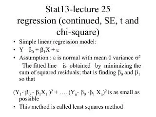
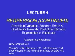
LECTURE 4 REGRESSION (CONTINUED) Analysis of Variance; Standard Errors & Confidence Intervals; Prediction Intervals; Examination of Residuals Supplementary Readings: Wilks, chapters 6,9; Bevington, P.R., Robinson, D.K., Data Reduction and Error Analysis for the Physical Sciences, McGraw-Hill, 1992.
Define: Recall from last time… We call these residuals What should we require of them?
GAUSSIAN Recall from last time… What should we require of them?
Recall from last time… Analysis of Variance (“ANOVA”)? 2(n=5) Gaussian data
is guaranteed by linear regression procedure Analysis of Variance (“ANOVA”) Why “n-2”?
Analysis of Variance (“ANOVA”) Define:
Analysis of Variance (“ANOVA”) Define:
Analysis of Variance (“ANOVA”) 1 and n-2 degrees of freedom
Analysis of Variance (“ANOVA”) Source df SS MS F-test Total n-1 SST Regression 1 SSR MSR=SSR MSR/MSE Residual n-2 SSE MSE=se2 1 and n-2 degrees of freedom
Analysis of Variance (“ANOVA”) for Simple Linear Regression Source df SS MS F-test Total n-1 SST Regression 1 SSR MSR=SSR MSR/MSE Residual n-2 SSE MSE=se2 We’ll discuss ANOVA further in the next lecture (“multivariate regression”)
If we have: ‘Goodness of Fit’ Linear Correlation
‘Goodness of Fit’ For simple linear regression
‘Goodness of Fit’ Outside the “support” of the regression, in general,
‘Goodness of Fit’ Outside the “support” of the regression, in general,
‘Goodness of Fit’ Reliability Bias
‘Goodness of Fit’ Reliability Bias
Analysis of Variance (“ANOVA”) Under Gaussian assumptions, the estimates from linear regression of the parameter a and b represent unbiased estimates of means of a Gaussian distribution Where the standard errors in the regression parameters are:
Confidence Intervals The estimated regression slope ‘b’ is likely to be within some range of the true ‘b’
Confidence Intervals This naturally defines a t test for the presence of a trend:
Prediction Intervals MSE in a predicted value or, (‘Prediction Error’) is larger than the nominal MSE, increasing as the predictand value departs from the mean Note that sy approaches se as the ‘training’ sample becomes large
Linear Correlation ‘r’ suffers from sampling error both in the regression slope and the estimates of variance…
Linear Correlation ‘r’ suffers from sampling error both in the regression slope and the estimates of variance…
Examining Residuals Heteroscedasticity A trend in residual variance violates the assumption of Gaussian residuals…
Examining Residuals Heteroscedasticity Often a simple transformation of the original data will yield more closely Gaussian residuals…
Examining Residuals Leverage Points can still be a problem!
Examining Residuals Autocorrelation Durbin-Watson Statistic
Suppose we have the simple (‘first order autoregressive’) model For example: Examining Residuals Autocorrelation Then we can still use all of the results based on Gaussian statistics, but with the modified sample size:
Suppose we have the simple (‘first order autoregressive’) model Examining Residuals Autocorrelation Then we can still use all of the results based on Gaussian statistics, but with the modified sample size: Different for tests of variance
Suppose we have the simple (‘first order autoregressive’) model Examining Residuals Autocorrelation Then we can still use all of the results based on Gaussian statistics, but with the modified sample size: Different again for correlations
Suppose we have the simple (‘first order autoregressive’) model Examining Residuals We can remove the serial correlation through
Autocorrelation AR(1) PROCESS For simplicity, we will assume zero mean
Autocorrelation AR(1) PROCESS What is the standard deviation of an AR(1) process?
Using, Autocorrelation AR(1) PROCESS Recursively, we thus have for an AR(1) process, For a long series, the sampling distribution for r is approximately Gaussian (like the slope parameter in linear regression), with standard deviation, How do we determine if r is significantly non-zero?
Autocorrelation This is essentially the t test statistic Example: consider the case r=0.2, n=200 Z=0.2/(0.96/200)1/2 =0.2/0.069=2.9 This is approximately the 3 sigma level of a Gaussian distribution. p=0.004 for a two-sided test, p=0.002 for a one-sided test