Understanding Histograms: Construction, Interpretation, and Common Shapes
This guide covers the key differences between histograms and bar charts, focusing on the construction and interpretation of histograms from raw data. Learn the process to categorize data into classes, determine class widths, midpoints, and boundaries, and understand how to sketch the histogram effectively. We also explore relative frequency, cumulative frequency, and recognize various shapes of histograms, including symmetrical, skewed, and bimodal. Ideal for students and professionals seeking a comprehensive overview of histogram representation in statistics.

Understanding Histograms: Construction, Interpretation, and Common Shapes
E N D
Presentation Transcript
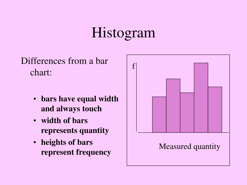
Histogram Differences from a bar chart: • bars have equal width and always touch • width of bars represents quantity • heights of bars represent frequency f Measured quantity
To construct a histogram from raw data: • Decide on the number of classes (5 to 15 is customary). • Find a convenient class width. • Organize the data into a frequency table. • Find the class midpoints and the class boundaries. • Sketch the histogram.
Finding class width 1. Compute: 2. Increase the value computed to the next highest whole number
Raw Data: 10.2 18.7 22.3 20.0 6.3 17.8 17.1 5.0 2.4 7.9 0.3 2.5 8.5 12.5 21.4 16.5 0.4 5.2 4.1 14.3 19.5 22.5 0.0 24.7 11.4 Use 5 classes. 24.7 – 0.0 5 = 4.94 Round class width up to 5. Class Width
Frequency Table • Determine class width. • Create the classes. May use smallest data value as lower limit of first class and add width to get lower limit of next class. • Tally data into classes. • Compute midpoints for each class. • Determine class boundaries.
Tallying the Data # of miles tally frequency 0.0 - 4.9 |||| | 6 5.0 - 9.9 |||| 5 10.0 - 14.9 |||| 4 15.0 - 19.9 |||| 5 20.0 - 24.9 |||| 5
Grouped Frequency Table # of miles f 0.0 - 4.9 6 5.0 - 9.9 5 10.0 - 14.9 4 15.0 - 19.9 5 20.0 - 24.9 5 Class limits: lower - upper
Computing Class Width difference between the lower class limit of one class and the lower class limit of the next class
Finding Class Widths # of miles f class widths 0.0 - 4.9 6 5 5.0 - 9.9 6 5 10.0 - 14.9 4 5 15.0 - 19.9 5 5 20.0 - 24.9 5 5
Computing Class Midpoints lower class limit + upper class limit 2
Finding Class Midpoints # of miles f class midpoints 0.0 - 4.9 6 2.45 5.0 - 9.9 5 10.0 - 14.9 4 15.0 - 19.9 5 20.0 - 24.9 5
Finding Class Midpoints # of miles f class midpoints 0.0 - 4.9 6 2.45 5.0 - 9.9 5 7.45 10.0 - 14.9 4 15.0 - 19.9 5 20.0 - 24.9 5
Finding Class Midpoints # of miles f class midpoints 0.0 - 4.9 6 2.45 5.0 - 9.9 5 7.45 10.0 - 14.9 4 12.45 15.0 - 19.9 5 17.45 20.0 - 24.9 5 22.45
Class Boundaries (Upper limit of one class + lower limit of next class) divided by two
Finding Class Boundaries # of miles f class boundaries 0.0 - 4.9 6 5.0 - 9.9 5 4.95 - 9.95 10.0 - 14.9 4 15.0 - 19.9 5 20.0 - 24.9 5
Finding Class Boundaries # of miles f class boundaries 0.0 - 4.9 6 5.0 - 9.9 5 4.95 - 9.95 10.0 - 14.9 4 9.95 - 14.95 15.0 - 19.9 5 20.0 - 24.9 5
Finding Class Boundaries # of miles f class boundaries 0.0 - 4.9 6 5.0 - 9.9 5 4.95 - 9.95 10.0 - 14.9 4 9.95 - 14.95 15.0 - 19.9 5 14.95 - 19.95 20.0 - 24.9 5
Finding Class Boundaries # of miles f class boundaries 0.0 - 4.9 6 ?? 5.0 - 9.9 5 4.95 - 9.95 10.0 - 14.9 4 9.95 - 14.95 15.0 - 19.9 5 14.95 - 19.95 20.0 - 24.9 5 19.95 - 24.95
Finding Class Boundaries # of miles f class boundaries 0.0 - 4.9 6 ?? - 4.95 5.0 - 9.9 5 4.95 - 9.95 10.0 - 14.9 4 9.95 - 14.95 15.0 - 19.9 5 14.95 - 19.95 20.0 - 24.9 5 19.95 - 24.95
Finding Class Boundaries # of miles f class boundaries 0.0 - 4.9 6 0.05 - 4.95 5.0 - 9.9 5 4.95 - 9.95 10.0 - 14.9 4 9.95 - 14.95 15.0 - 19.9 5 14.95 - 19.95 20.0 - 24.9 5 19.95 - 24.95
6 5 4 3 2 1 0 - - - - - - - | | | | | | -0.05 4.95 9.95 14.95 19.95 24.95 mi. Constructing the Histogram f # of miles f 0.0 - 4.9 6 5.0 - 9.9 5 10.0 - 14.9 4 15.0 - 19.9 5 20.0 - 24.9 5
Relative Frequency Relative frequency = f = class frequency n total of all frequencies
Relative Frequency f = 6 = 0.24 n 25 f = 5 = 0.20 n 25
.24 .20 .16 .12 .08 .04 0 - - - - - - - Relative frequency f/n | | | | | | -0.05 4.95 9.95 14.95 19.95 24.95 mi. Relative Frequency Histogram # of miles f relative frequency 0.0 - 4.9 6 0.24 5.0 - 9.9 5 0.20 10.0 - 14.9 4 0.16 15.0 - 19.9 5 0.20 20.0 - 24.9 5 0.20
Common Shapes of Histograms When folded vertically, both sides are (more or less) the same. Symmetrical f
Common Shapes of Histograms Also Symmetrical f
Common Shapes of Histograms Uniform f
Common Shapes of Histograms Non-Symmetrical Histograms These histograms areskewed.
Common Shapes of Histograms Skewed Histograms Skewedleft Skewed right
Common Shapes of Histograms Bimodal f The two largest rectangles are approximately equal in height and are separated by at least one class.
Frequency Polygon A frequency polygon or line graph emphasizes the continuous rise or fall of the frequencies.
Constructing the Frequency Polygon • Dots are placed over the midpoints of each class. • Dots are joined by line segments. • Zero frequency classes are included at each end.
Constructing the Frequency Polygon Weights (in pounds) f 2 - 4 6 5 - 7 5 8 - 10 4 11 - 13 5 f 6 5 4 3 2 1 0 - - - - - - - | | | | | | 0 3 6 9 12 15 pounds
Cumulative Frequency The sum of the frequencies for that class and all previous or later classes
Cumulative Frequency Table Weights (in pounds) f Greater than 1.5 20 Greater than 4.5 14 Greater than 7.5 9 Greater than 10.5 5 Greater than 13.5 0 Weights (in pounds) f 2 - 4 6 5 - 7 5 8 - 10 4 11 - 13 5 20
Ogive Graph of a cumulative frequency table
Constructing the Ogive Weights (in pounds) f Greater than 1.5 20 Greater than 4.5 14 Greater than 7.5 9 Greater than 10.5 5 Greater than 13.5 0 20 15 10 5 0 - - - - - Cumulative frequency | | | | | | 1.5 4.5 7.5 10.5 13.5 pounds
Exploratory Data Analysis • A field of statistical study useful in detecting patterns and extreme data values • Tools used include histograms and stem-and-leaf displays