Histogram
Histogram. Histogram is a graph that shows frequency of anything. Histograms usually have bars that represent frequency of occuring of data. Histogram has two axis: x and y. The x axis contains the event whose frequency we count. The y axis contains frequency. Histogram.

Histogram
E N D
Presentation Transcript
Histogram • Histogram is a graph that shows frequency of anything. Histograms usually have bars that represent frequency of occuring of data. • Histogram has two axis: x and y. • The x axis contains the event whose frequency we count. • The y axis contains frequency.
Histogram • Example of a typical histogram.
Histogram • Consider some students with their marks.
Image histogram • Image histogram shows frequency of pixel intensity values. • x axis shows the gray level intensities • y axis shows the frequency of intensities.
Image histogram x axis – shows the range of pixel values. For 8 bpp image, we have 256 levels of gray shades
Brightness • Brightness is a relative term. It can be defined as the amount of energy output by a source of light relative to the source we are comparing to. Image on the right is brighter than image on the left.
Brightness • Brightness can be easily increased or decreased by simple addition or subtraction to the image matrix
Contrast • The contrast of the image can be defined as the difference between maximum pixel intensity and minimum pixel intensity. • Max. int. = 0, Min. int. =0 • Contrast = 0–0=0 • Max. int. = 100, Min. int. =100 • Contrast = 100–100=0
Image transformations • Transformation is a function. It maps one set to another set after performing some operations. • Digital Image Processing system performs the transformation.
Image transformation • Consider the equation g(x,y)=T(f(x,y)) f(x,y) – input image, transformation is applied to this image. g(x,y) – output image (processed image). T is a transformation function.
Image transformation • The transformation can be also represented as s=T(r) r – pixel value of the input image f(x,y) s – pixel value of the output image g(x,y)
Image transformation Original image
Histogram sliding • Brightness is changed by shifting the histogram to left or right. +50
Histogram sliding - 30
Histogram stretching • Contrast can be increased using: 1. Histogram stretching 2. Histogram equalization • Contrast is the difference between maximum and minimum pixel intensity. Contrast = 225.
Increasing the contrast f(x,y) g(x,y) Low contrast image High contrast image
Contrast stretching Before Contrast = 225 After Contrast = 240
Contrast stretching • This formula doesn’t work always. If there is 1 pixel with intensity 255: Contrast stretching has no effect!!!
Introduction to probability • PMF and CDF are both related to probability. They will be used in Histogram Equalization. • PMF – Probability Mass Function. • It gives the probability of each number in the data set (frequency of each element).
Probability – PMF Calculating PMF from image matrix PMF Image matrix 1 2 7 5 6 7 2 3 4 5 0 1 5 7 3 1 2 5 6 7 6 1 0 3 4
Probability – PMF Calculating PMF from histogram Frequency of gray level values for an 8 bits per pixel image. Not monotonically increasing function
Probability – CDF • CDF – Cumulative Distributed Function • Cumulative sum of values calculated by PMF
Probability – CDF • CDF will be calculated using the histogram • CDF makes the PDF grow monotonically • Monotonical growth is necessary for histogram equalization.
Histogram equalization • Histogram equalization is used for enhancing the contrast of the images. • The first two steps are calculating the PDF and CDF. • All pixel values of the image will be equalized.
Histogram equalization • Image with its histogram
Histogram equalization Small image (values) Small image (values)
Histogram equalization Image detail Frequency of pixel values
Histogram equalization • min = 52 • max = 154 cdfmin is the minimum non-zero value of the cumulative distribution function (in this case 1), M × N gives the image's number of pixels (for the example above 64, where M is width and N the height) and L is the number of grey levels used (in most cases, like this one, 256).
Histogram equalization New min. value = 0, old min. value 52 New max. value = 255, old max. value 154 Original Equalized
Histogram equalization Corresponding histogram (red) and cumulative histogram (black) An unequalized image The same image after histogram equalization Corresponding histogram (red) and cumulative histogram (black)
Negative transformation Negative Original s = (L – 1) – r
Concept of convolution Black box
Concept of convolution g(x,y) = h(x,y) * f(x,y) mask convolved with an image g(x,y) = f(x,y) * h(x,y)image convolved with mask The convolution operator (*) is commutative, h(x,y) is the mask or filter.
Convolution mask • Mask is a matrix, usually of size 1x1, 3x3, 5x5 or 7x7 (odd number). • Convolution steps: • Flip the mask horizontally and vertically • Slide the mask onto the image • Multiply the corresponding elements and add them • Repeat this until all image values are calculated
Convolution example • Mask: • After flipping the mask:
Convolution example • Image matrix • Place the mask over each image element. Multiply the corresponding elements and add them
Convolution example • Red – mask, black – image • First pixel: = (5*2) + (4*4) + (2*8) + (1*10) • = 10 + 16 + 16 + 10 • = 52 • Convolution can achieve blurring, edge detection, sharpening, noise reduction, etc
Concept of mask • A mask is a filter. Concept of masking is a concept of spatial filtering. • Sample mask • Filtering is convolving a mask with an image by moving the center of the mask over each image pixel.
Filters • Filters are used for: - blurring - noise reduction - image sharpening - edge detection