Download
1 / 39
390 likes | 584 Views
The pipe junction challenge. Tor Dokken SINTEF Oslo, Norway Pictures and examples by Vibeke Skytt, SINTEF. What is a pipe junction?. A composition of cylindrical pipes meeting. For structural use the pipes are welded without cut-outs

E N D
The pipe junction challenge Tor Dokken SINTEF Oslo, Norway Pictures and examples by Vibeke Skytt, SINTEF
What is a pipe junction? • A composition of cylindrical pipes meeting. • For structural use the pipes are welded without cut-outs • For use for transport of fluids or gas, cut-outs are made. • Welding seams smooth the transition between pipes (fillet volumes)
How to represent the pipe-junction in the computer The representation approach depends on the application domain (the purpose of the computer program): • Visualization of the model • Animation of the model • Design of the model • Production of the model • Analysis of the model, and type of analysis • Structural, flow,…
Example of pipe junction from the age of curved based CAD, • Example from the mid 1970s of the geometry of cylinder junction from an offshore platform in the oil industry. • Cylinders made from steel plates, one cylinder is flattend for flame cutting. • Accurate geometry of cut-outs important. • Flame cutters controlled by curve data. • In current industry welding robots plays a central role • Robots controlled by curve data • Navigation of robots need an approximate surface based model for collision detection and navigation.
Representation of the pipe junction for design and analysis • Target quality criteria for this presentation: • Design stage: Face connectivity + Shape accuracy • Analysis stage: Volumetric connectivity + Shape accuracy • The ideal pipe junction can be composed of pieces of cylindrical tubes. • During structural analysis loads are applied to the structures, the shape will be deflected becoming slightly sculptured • NURBS* used in CAD for representing sculptured surfaces • NURBS used in isogeometric analysis for representing sculptured volumes • *NURBS - NonUniform Rational B-splines
Elementary surfaces play a central role in human made structures • Elementary surfaces dominates design of modern human made industrial produced shapes: • Plane • Cylinder • Sphere • Cone • Torus • Surfaces of more sculptured type relates to • Terrain • Actual shape of produced parts (elementary shapes slightly deflected) • Styled and designed products • Shapes made by artists • Vegetation is in general fractal
Some properties of elementary surfaces • Elementary surfaces all have an exact rational parameterization • The deflected elementary surface can be efficiently approximated by a NURBS-surface or by an algebraic surface of somewhat higher degree • Elementary surfaces have low algebraic degree: • Degree 1: Plane • Degree 2: Cylinder, Sphere, Cone • Degree 4: Torus • Algorithms for handling elementary surfaces can both use the algebraic and rational parametric representation
Design representation - Volumetric CAD – Boundary structures (STEP ISO 10303) • Representation of outer and inner hulls by surface patchwork • Small gaps between surface allowed • Edges of NURBS surfaces represented by 3 curves: • A 3D curve • One curve in the parameter domain of each NURBS surface • Each of the 3 curves is an approximations of the exact edge curve
Why a volume structure? • Parametric NURBS surfaces without trimming (curves removing parts of the domain) have 4 edge curves. • Parametric NURBS volumes have 6 outer faces and is the mapping of an axis parallel box in the parameter domain.
Elementary shapes are not so simple as we used to think. Why? • Isogeometric analysis allows in principle direct coupling of CAD and FEA. However, • The models are respectively 2-variate and 3-variate, model restructuring necessary • The elementary surface of CAD has to be given a suitable NURBS representation • The CAD approach of 3 version of intersection curves cannot be allowed • Isogeometric analysis demands accurate tri-variate parametric representations of the objects to be analyzed. • No gaps allowed unless they reflect the actual geometry (e.g., a crack in the object).
Independent evolution of CAD and Finit Element Analysis (FEA) • CAD (NURBS) and Finite Element Analysis evolved in different communities before electronic data exchange • FEM developed to improve analysis in Engineering • CAD developed to improve the design process • Information exchange was drawing based, consequently the mathematical representation used posed no problems • Manual modelling of the element grid • Implementations used approaches that best exploited the limited computational resources and memory available. • FEA was developed before the NURBS theory • FEA evolution started in the 1940s and was given a rigorous mathematical foundation around 1970 (E.g, ,1973: Strang and Fix's An Analysis of The Finite Element Method) • B-splines: 1972: DeBoor-Cox Calculation, 1980: Oslo Algorithm
Why are splines important to isogeometric analysis? • Splines are polynomial, same as Finite Elements • B-Splines are very stable numerically • B-splines represent regular piecewise polynomial structure in a more compact way than Finite Elements • NonUniform rational B-splines can represent elementary curves and surfaces exactly. (Circle, ellipse, cylinder, cone…) • Efficient and stable methods exist for refining the piecewise polynomials represented by splines • Knot insertion (Oslo Algorithm, 1980, Cohen, Lyche, Riesenfeld) • B-spline has a rich set of refinement methods
Challenge 1: Topology • How to split the object into proper 3-variate parametric NURBS
Steps in making the NURBS volume • Calculate the intersection of the cylinders. • Subdivide the cylinders into four sided regions by superimposing an edge and vertex structure • The only situation when C1 continuity is simple is when a vertex has 4 vertices, and opposing edges across the vertex meet with proper C1 continuity. • The regions should be made to simplify the making of the NURBS surfaces, and C1 or higher continuity between surfaces.
In more detail 1. 1 2 • Construct two pipes, 1 and 2 • Intersect 1 and 2, selecting the boundary piece of 1 as intersection surface • Trim 2 • Trim the boundary of 1 • Adapt 2 to the new boundary information to remove trimming • Split 1 to remove boundary trimming • Split 2 to meet the volumes originating from 1 corner-to-corner • Update topology for each step • Ensure continuity along boundary surfaces
In more detail 2. Parameter domain of boundary surface of volume 1 • Ruled based approach • Volume 1 touches the updated volume 2 along the white ring • Splitting will be performed along the dotted lines • The inner circle will get corner singularities • Approximation is required as the geometry is not planar • The topology of the split will be uniform in the thickness direction, i.e. the volume is split as the surface • 14 blocks for volume 1 • 4 blocks for volume 2
Construction of pipe junction • Two pipes represented as spline volumes • We want to make a block structured isogeometric model • Initial method: Boolean operations on volumes
Intersecting all boundary surfaces • The boundary surfaces of one volume are not suited for the topology structure due to two surfaces along the seam • The method is partly based on stable SISL intersections and partially on experimental or prototype GoTools code • Tolerance issues: Accuracy versus data size • Surface types: The method expects spline surfaces, but the boundary surfaces are SurfaceOnVolume
Splitting the initial models Pipe 1 Pipe 2
Modifying pipe 2 • The outer part of the pipe is selected • One boundary surface is fetched from pipe 1 • This boundary surface must be approximated within the spline space of the initial volume • Modification/construction of volume • Adapt the volume to the new boundary surface. Volume smoothing is used • Recreate the volume by linear loft between the new and the initial end surface • Create volume interpolating all boundary surfaces (Coons approach)
The middle part Extra boundary surfaces extracted from the boundary surfaces of pipe 1
Pipe 1 • This volume gets a hole by the Boolean operation • Lets consider the outer cylinder surface • Split the trimmed surface to get 4-sided surfaces that can be represented by spline surfaces
Challenge 2: Geometry • Representation by rational parametric • Curves • Surfaces • Volumes
The intersection of two cylinders • Let the first cylinders be represented implicitly: • The centre c • A unit vector d specifying the direction of the axis • The radius The implicit description of the cylinder is then • Let the second cylinder have radius 1, and have the z-axis as its axis, and let a quarter be described by the rational parameterization
Combining the cylinders • Inserting the parametric represented cylinder in the implicit represented cylinder yields a polynomial of total degree 4, up to degree 4 in u and up to degree 2 in v • This is an algebraic curve of total degree 4 in u and v. • The general degree 4 algebraic curve do not have a rational parameterization, and this is the case for the cylinders when they are in general positions.
Approximation of shape cannot be avoided! • Two components contribute to the need for approximation • The intersection of two cylinders cannot in the general case be represented by a rational parameterization • The block structuring might impose shape approximation to work properly • Which approximation qualities are important? • Approximation error • Approximation ensured to be inside or outside of the real object • Distribution of the error • Degrees of the NURBS approximation • Ensure that approximation lies in one of the cylinders • The oscillatory behaviour of the approximation
Error when controlling tangent lengths cubic in Hermit interpolation • Simplest power expansion of tangents • Outside error Radius 1, opening angle 1
More examples • Near near equioscillating • Frist second and third derivate of error zero at midpoint
And even more examples • Error with zero integral q(p(t)) • Error when square sum of Bezier coefficients is minimal
Summery of methods • Examples from my doctorate thesis from 1997, that can be found at http://www.sintef.no/IST_GAIA menu the GAIA project. • (94, 95,… in the table refers to page numbers in the thesis)
Some shape approximation challenges • Curve level: Controlling the quality of the approximation of the intersection curve of two cylinders: • Cubic or higher degree polynomial approximation • Rational approximation • Surface level: Approximating the cylinder pieces resulting from segmentation of the trimmed cylinder in rectangular regions • Volume level: Approximating the tube segments resulting from the segmentation
Example smoothing of NURBS volume parameterization Video Courtesy: Kjell-Fredrik Pettersen, SINTEF
Challenge 3: Blends • Often the transition between cylinders is made smooth by adding blends. • Fillets can, e.g., represent grinded welds resulting from the manufacturing process. • The simplest way of making the blend is by rolling a ball that touch both cylinders, and using the surface traced out as the outer surface of the blend volume.
SAGA already addresses some blend surfaces • Heidi is addressing new approaches for making the fillet surface between a plane and cone together with Rimas. • I hope a next step is that we can address the fillet volume between the fillet surface, the cone and the plane. • A following challenge can the be to address the fillet volume between two cylinders and the fillet surface