Sigurd Skogestad , Vladimiros Minasidis, Julian Straus Department of Chemical Engineering

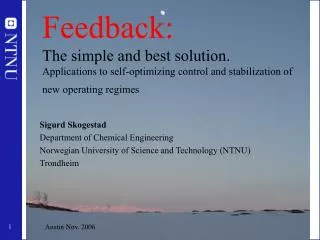
1. Economic plantwide controlThe critical link in integrated decision making across process operation Sigurd Skogestad, Vladimiros Minasidis, Julian Straus Department of Chemical Engineering Norwegian University of Science and Tecnology (NTNU) Trondheim, Norway Rhodes, Greece, 20 June 2016 TexPoint fonts used in EMF. Read the TexPoint manual before you delete this box.: AAA

2. Outline part1 • Objectives of control • Our paradigm • Planwide control procedure based on economics • Active constraints • Example: Runner • Selection of primary controlled variables (CV1=H y) • Optimal is gradient, CV1=Ju with setpoint=0 • General CV1=Hy. Nullspace and exact local method • Throughput manipulator (TPM) location • Example: Distillation • Active constraints regions • Example: Recycle plants

3. How we design a control system for a complete chemical plant? Where do we start? What should we control? and why? etc. etc.

4. In theory: Optimal control and operation Objectives Approach: • Model of overall system • Estimate present state • Optimize all degrees of freedom Process control: • Excellent candidate for centralized control Problems: • Model not available • Objectives = ? • Optimization complex • Not robust (difficult to handle uncertainty) • Slow response time CENTRALIZED OPTIMIZER Present state Model of system (Physical) Degrees of freedom

5. Optimal centralized Solution (EMPC) Academic process control community fish pond Sigurd

6. Practice: Engineering systems • Most (all?) large-scale engineering systems are controlled using hierarchies of quite simple controllers • Large-scale chemical plant (refinery) • Commercial aircraft • 100’s of loops • Simple components: PI-control + selectors + cascade + nonlinear fixes + some feedforward Same in biological systems But: Not well understood

7. Alan Foss (“Critique of chemical process control theory”, AIChE Journal,1973): The central issue to be resolved ... is the determination of control system structure. Which variables should be measured, which inputs should be manipulated and which links should be made between the two sets? There is more than a suspicion that the work of a genius is needed here, for without it the control configuration problem will likely remain in a primitive, hazily stated and wholly unmanageable form. The gap is present indeed, but contrary to the views of many, it is the theoretician who must close it. Previous work on plantwide control: • Page Buckley (1964) - Chapter on “Overall process control” (still industrial practice) • Greg Shinskey (1967) – process control systems • Alan Foss (1973) - control system structure • Bill Luyben et al. (1975- ) – case studies ; “snowball effect” • George Stephanopoulos and Manfred Morari (1980) – synthesis of control structures for chemical processes • Ruel Shinnar (1981- ) - “dominant variables” • Jim Downs (1991) - Tennessee Eastman challenge problem • Larsson and Skogestad (2000): Review of plantwide control

8. Main objectives control system • Economics: Implementation of acceptable (near-optimal) operation • Regulation: Stable operation ARE THESE OBJECTIVES CONFLICTING? • Usually NOT • Different time scales • Stabilization fast time scale • Stabilization doesn’t “use up” any degrees of freedom • Reference value (setpoint) available for layer above • But it “uses up” part of the time window (frequency range)

9. Our Paradigm Practical operation: Hierarchical structure Manager Planning constraints, prices Process engineer constraints, prices Operator/RTO setpoints Operator/”Advanced control”/MPC setpoints PID-control u = valves

10. Dealing with complexity Plantwide control: Objectives OBJECTIVE Min J (economics) RTO CV1s Follow path (+ look after other variables) MPC CV2s Stabilize + avoid drift PID u (valves) The controlled variables (CVs) interconnect the layers CV = controlled variable (with setpoint)

11. Optimizer (RTO) Optimally constant valves Always active constraints Supervisory controller (MPC) Regulatory controller (PID) H H2 Physical inputs (valves) d y PROCESS Stabilized process ny CV1s CV1 CV2s CV2 Degrees of freedom for optimization (usually steady-state DOFs), MVopt = CV1s Degrees of freedom for supervisory control, MV1=CV2s + unused valves Physical degrees of freedom for stabilizing control, MV2 = valves (dynamic process inputs)

12. Control structure design procedure I Top Down (mainly steady-state economics, y1) • Step 1: Define operational objectives (optimal operation) • Cost function J (to be minimized) • Operational constraints • Step 2: Identify degrees of freedom (MVs) and optimize for expected disturbances • Identify Active constraints • Step 3: Select primary “economic” controlled variables c=y1 (CV1s) • Self-optimizing variables (find H) • Step 4: Where locate the throughput manipulator (TPM)? II Bottom Up (dynamics, y2) • Step 5: Regulatory / stabilizing control (PID layer) • What more to control (y2; local CV2s)? Find H2 • Pairing of inputs and outputs • Step 6: Supervisory control (MPC layer) • Step 7: Real-time optimization (Do we need it?) y1 y2 MVs Process S. Skogestad, ``Control structure design for complete chemical plants'', Computers and Chemical Engineering, 28 (1-2), 219-234 (2004).

13. Step 1. Define optimal operation (economics) • What are we going to use our degrees of freedom u(MVs) for? • Define scalar cost function J(u,x,d) • u: degrees of freedom (usually steady-state) • d: disturbances • x: states (internal variables) Typical cost function: • Optimize operation with respect to u for given d (usually steady-state): minu J(u,x,d) subject to: Model equations: f(u,x,d) = 0 Operational constraints: g(u,x,d) < 0 J = cost feed + cost energy – value products

14. Step S2. Optimize(a) Identify degrees of freedom (b) Optimize for expected disturbances • Need good model, usually steady-state • Optimization is time consuming! But it is offline • Main goal: Identify ACTIVE CONSTRAINTS • A good engineer can often guess the active constraints

15. Step S3: Implementation of optimal operation • Have found the optimal way of operation. How should it be implemented? • What to control ? (primary CV’s). • Active constraints • Self-optimizing variables (for unconstrained degrees of freedom)

16. Optimal operation - Runner Optimal operation of runner • Cost to be minimized, J=T • One degree of freedom (u=power) • What should we control?

17. Optimal operation - Runner 1. Optimal operation of Sprinter • 100m. J=T • Active constraint control: • Maximum speed (”no thinking required”) • CV = power (at max)

18. Optimal operation - Runner 2. Optimal operation of Marathon runner • 40 km. J=T • What should we control? CV=? • Unconstrained optimum J=T u=power uopt

19. Optimal operation - Runner Self-optimizing control: Marathon (40 km) • Any self-optimizing variable (to control at constant setpoint)? • c1 = distance to leader of race • c2 = speed • c3 = heart rate • c4 = level of lactate in muscles

20. Optimal operation - Runner Conclusion Marathon runner select one measurement c = heart rate J=T • CV = heart rate is good “self-optimizing” variable • Simple and robust implementation • Disturbances are indirectly handled by keeping a constant heart rate • May have infrequent adjustment of setpoint (cs) c=heart rate copt

21. Step 3. What should we control (c)? Selection of primary controlled variables y1=c • Control active constraints! • Unconstrained variables: Control self-optimizing variables! • Old idea (Morariet al., 1980): “We want to find a function c of the process variables which when held constant, leads automatically to the optimal adjustments of the manipulated variables, and with it, the optimal operating conditions.”

22. Unconstrained degrees of freedom The ideal “self-optimizing” variable is the gradient, Ju c =  J/ u = Ju Keep gradient at zero for all disturbances (c = Ju=0) Problem: Usually no measurement of gradient Ju<0 cost J uopt Ju<0 0 Ju Ju=0 u

23. Never try to control the cost function J (or any other variable that reaches a maximum or minimum at the optimum) • Better: control its gradient, Ju, or an associated “self-optimizing” variable. J>Jmin ? Jmin J<Jmin Infeasible J u

24. Good Good BAD General: What variable c=Hy should we control? (for self-optimizing control) • The optimal value of c should be insensitive to disturbances • Small Fc = dcopt/dd • c should be easy to measure and control • Want “flat” optimum -> The value of c should be sensitive to changes in the degrees of freedom (“large gain”) • Large G = dc/du = HGy Note: Must alsofind optimal setpoint for c=CV1

25. Nullspace method • Proof. Appendix B in: Jäschke and Skogestad, ”NCO tracking and self-optimizing control in the context of real-time optimization”, Journal of Process Control, 1407-1416 (2011) • .

26. With measurement noise More general (“exact local method”) • No measurement error: HF=0 (nullspace method) • With measuremeng error: Minimize GFc • Maximum gain rule

27. Example. Nullspace Method for Marathon runner u = power, d = slope [degrees] y1 = hr [beat/min], y2 = v [m/s] F = dyopt/dd = [0.25 -0.2]’ H = [h1 h2]] HF = 0 -> h1 f1 + h2 f2 = 0.25 h1 – 0.2 h2 = 0 Choose h1 = 1 -> h2 = 0.25/0.2 = 1.25 Conclusion: c = hr + 1.25 v Control c = constant -> hr increases when v decreases (OK uphill!)

28. Step 4. Where set production rate? • Where locale the TPM (throughput manipulator)? • The ”gas pedal” of theprocess • Very important! • Determines structure of remaining inventory (level) control system • Set production rate at (dynamic) bottleneck • Link between Top-down and Bottom-up parts • NOTE: TPM location is a dynamic issue. Link to economics is to improve control of active constraints (reduce backoff)

29. Production rate set at inlet :Inventory control in direction of flow* TPM * Required to get “local-consistent” inventory control

30. Production rate set at outlet:Inventory control opposite flow TPM

31. Production rate set inside process TPM Radiating inventory control around TPM (Georgakis et al.)

32. Operation of Distillation columns in series Example /QUIZ 1 • Cost (J) = - Profit = pF F + pV(V1+V2) – pD1D1 – pD2D2 – pB2B2 • Prices: pF=pD1=PB2=1 $/mol, pD2=2 $/mol, Energy pV= 0-0.2 $/mol (varies) • With given feed and pressures: 4 steady-state DOFs. • Here: 5 constraints (3 products > 95% + 2 capacity constraints on V) = N=41 αAB=1.33 N=41 αBC=1.5 > 95% A pD1=1 $/mol > 95% B pD2=2 $/mol F ~ 1.2mol/s pF=1 $/mol = = < 4 mol/s < 2.4 mol/s > 95% C pB2=1 $/mol QUIZ: What are the expected active constraints? 1. Always. 2. For low energy prices. DOF = Degree Of Freedom Ref.: M.G. Jacobsen and S. Skogestad (2011)

33. SOLUTION QUIZ1 + new QUIZ2 Control of Distillation columns in series xB CC xBS=95% PC PC LC LC Quiz2: UNCONSTRAINED CV=? Given MAX V2 MAX V1 LC LC Red: Basic regulatory loops

34. Solution. xB xB CC CC xBS=95% xAS=2.1% Control of Distillation columns. Cheap energy PC PC LC LC Given MAX V2 MAX V1 LC LC

35. Distillation example: Not so simple Active constraint regions for two distillation columns in series 0 1 Mode 1 (expensive energy) Energy price 1 Mode 2: operate at BOTTLENECK. F=1,49 Higher F infeasible because all 5 constraints reached [$/mol] 2 0 2 3 1 [mol/s] Mode 1, Cheap energy: 3 active constraints -> 1 remaining unconstrained DOF (L1) -> Need to find 1 additional CVs (“self-optimizing”) More expensive energy: Only 1 active constraint (xB) ->3 remaining unconstrained DOFs -> Need to find 3 additional CVs (“self-optimizing”) CV = Controlled Variable

36. How many active constraints regions? Distillation nc = 5 25 = 32 xB always active 2^4 = 16 -1 = 15 In practice = 8 • Maximum: nc = number of constraints BUT there are usually fewer in practice • Certain constraints are always active (reduces effective nc) • Only nu can be active at a given time nu = number of MVs (inputs) • Certain constraints combinations are not possibe • For example, max and min on the same variable (e.g. flow) • Certain regions are not reached by the assumed disturbance set

37. CV = Active constraint D1 xB Example back-off. xB = purity product > 95% (min.) • D1 directly to customer (hard constraint) • Measurement error (bias): 1% • Control error (variation due to poor control): 2% • Backoff = 1% + 2% = 3% • Setpoint xBs= 95 + 3% = 98% (to be safe) • Can reduce backoff with better control (“squeeze and shift”) • D1 to large mixing tank (soft constraint) • Measurement error (bias): 1% • Backoff = 1% • Setpoint xBs= 95 + 1% = 96% (to be safe) • Do not need to include control error because it averages out in tank xB xB,product ±2% 8

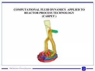
38. Case study: Recycle plant CSTR 1st order kinetics (undesired) Column • 30 stages • LV - configuration • Assumptions: • Constant relative volatilities • Constant molar overflows • Constant pressure Based on Luyben. Details can be found in Jacobsen et. al, [2011] V. Minasidis et al, Automated Controlled Variable Selection for a Reactor-Separator-Recycle Process

39. Step 1: Defineoperationalobjectives and degrees of freedom Cost function: steam cost value products cost feed prices in $/kmol Operational constraints*: Degrees of freedom (DOF): With given F: 4 steady state DOFs: Disturbances • Main disturbances: • Feed flow • Energy price V. Minasidis et al, Automated Controlled Variable Selection for a Reactor-Separator-Recycle Process Expected disturbance range ±30%

40. Step 2: Optimize (by gridding) Always active: 4 active constraints regions (with additional constraints): Bottleneck Operational constraints:

41. Summary so far:Systematic procedure for plantwide control • Start “top-down” with economics: • Step 1: Define operational objectives and identify degrees of freeedom • Step 2: Optimize steady-state operation. • Step 3A: Identify active constraints = primary CVs c. • Step 3B: Remaining unconstrained DOFs: Self-optimizing CVs c. • Step 4: Where to set the throughput (usually: feed) • Regulatory control I: Decide on how to move mass through the plant: • Step 5A: Propose “local-consistent” inventory (level) control structure. • Regulatory control II: “Bottom-up” stabilization of the plant • Step 5B: Control variables to stop “drift” (sensitive temperatures, pressures, ....) • Pair variables to avoid interaction and saturation • Finally: make link between “top-down” and “bottom up”. • Step 6: “Advanced/supervisory control” system (MPC): • CVs: Active constraints and self-optimizing economic variables + • look after variables in layer below (e.g., avoid saturation) • MVs: Setpoints to regulatory control layer. • Coordinates within units and possibly between units cs http://www.nt.ntnu.no/users/skoge/plantwide

42. Summary and references • The following paper summarizes the procedure: • S. Skogestad, ``Control structure design for complete chemical plants'', Computers and Chemical Engineering, 28 (1-2), 219-234 (2004). • There are many approaches to plantwide control as discussed in the following review paper: • T. Larsson and S. Skogestad, ``Plantwide control: A review and a new design procedure'' Modeling, Identification and Control, 21, 209-240 (2000). • The following paper updates the procedure: • S. Skogestad, ``Economic plantwide control’’, Book chapter in V. Kariwala and V.P. Rangaiah (Eds), Plant-Wide Control: Recent Developments and Applications”, Wiley (2012). • Another paper: • S. Skogestad “Plantwide control: the search for the self-optimizing control structure‘”, J. Proc. Control, 10, 487-507 (2000). • More information: http://www.nt.ntnu.no/users/skoge/plantwide

43. Part 2. Challenges and open problems(at least to me) • Oh yes 

44. Challenge: Effective plantwide optimization using detailed models Status • Offline: Optimization to findconstraintregions etc. is much more difficultthan I expected • Hopelesswith standard flowsheetingsoftware (Hysys, Aspen, Unisim, etc.) • VerydifficultalsowithMatlab, gProms, etc • Online: Even more difficult. RTO basedondetailedphysical has generallyfailed. Only used onethylene plants according to Honeywell (Joseph Lu, IFAC WC 2014, Cape Town) Challenges: • Effectiveoff-line optimization and generation of activeconstraints regions • Models thataresuited for optimization • «Surrogate» models RTO = Real-time optimization (steady state)

45. Challenge 1: Find active constraint regions Phase diagram = Active contraint region map Same topology as for «our» active constraint regions Phase «active»: Corresponding phase equilibrium equations are active, f=0

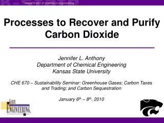
46. Challenge 1: Find active constraint regions CO2-stripper case study Matlab model

49. Challenge 2: Surrogate models suited for optimization 2. Surrogate steady-statemodels for efficient and accurateflowsheetoptimization • hysys/Aspen + standard optimization (build-in, Matlab/fmincon, Excel) is not working

50. 2. Surrogate steady-statemodels for efficient and accurateflowsheetoptimization • Unit by unit • Connections are linear, Out1 = In 2 • Main problem: Dimension too high • Independent variables: Fi + p,T for each feed stream + u’s (e.g. Q) + d’s • Dependent variables: Fi + p,T for each product stream • But: Need max. 4-6 independent variables for most surrogate models (table look-up, splines), (maybe may allow more for polynmials and neural nets ?? But I doubt it) • Suggested approach • First introduce material balances (linear) with extent of reaction as independent variable • Use PLS to find additional linear relationships • Remaining (including extent of reaction) nonlinear surrogate models • Must also reduce required range of variables (for gridding) • No need to generate data/samples in regions where the system will never operate. • To avoid this: Introduce change in independent variables, e.g. Q->T • Can base this in existing control structure (or more generally: self-optimizing control ideas)