Download
1 / 40
410 likes | 448 Views
The lecture slides focus on AI planning, covering conceptual models, planning algorithms, and successful applications in space exploration (NASA missions), manufacturing (sheet-metal bending machines), and games (computer bridge championships).

E N D
Artificial Intelligence Planning Gholamreza Ghassem-Sani Sharif University of Technology Lecture slides are mainly based on Dana Nau’s AI Planning University of Maryland
Related Reading • For technical details: • Malik Ghallab, Dan Nau, and Paolo TraversoAutomated Planning: Theory and PracticeMorgan Kaufmann, May 2004ISBN 1-55860-856-7 • Web site: • http://www.laas.fr/planning
Outline • Planning Successful Applications • Conceptual model for planning • Example planning algorithms
Planning Successful Applications • Space Exploration • Manufacturing • Games
Space Exploration • Autonomous planning, scheduling, control • NASA • Remote Agent Experiment (RAX) • Deep Space 1 • Mars ExplorationRover (MER)
Manufacturing • Sheet-metal bending machines - Amada Corporation • Software to plan the sequence of bends[Gupta and Bourne, J. Manufacturing Sci. and Engr., 1999]
Games • Bridge Baron - Great Game Products • 1997 world champion of computer bridge [Smith, Nau, and Throop, AI Magazine, 1998] • 2004: 2nd place Us:East declarer, West dummy Opponents:defenders, South & North Contract:East – 3NT On lead:West at trick 3 Finesse(P1; S) East:KJ74 West: A2 Out: QT98653 LeadLow(P1; S) FinesseTwo(P2; S) PlayCard(P1; S, R1) EasyFinesse(P2; S) StandardFinesse(P2; S) BustedFinesse(P2; S) … … West—2 (North—Q) (North—3) StandardFinesseTwo(P2; S) StandardFinesseThree(P3; S) FinesseFour(P4; S) PlayCard(P2; S, R2) PlayCard(P3; S, R3) PlayCard(P4; S, R4) PlayCard(P4; S, R4’) North—3 East—J South—5 South—Q
Conceptual Model1. Environment System State transition system = (S,A,E,)
s1 s0 put take location 2 location 1 location 2 location 1 move1 move2 move1 move2 s3 s2 put take location 2 location 2 location 1 location 1 load unload s4 s5 move2 move1 location 2 location 2 location 1 location 1 State Transition System = (S,A,E,) • S = {states} • A = {actions} • E = {exogenous events} • State-transition function: Sx (AE) 2S • S = {s0, …, s5} • A = {move1, move2, put, take, load, unload} • E = {} • : see the arrows The Dock Worker Robots (DWR) domain
s3 location 2 location 1 Conceptual Model2. Controller Given observation o in O, produces action a in A Controller Observation function h: SO State transition system = (S,A,E,)
s3 location 2 location 1 Conceptual Model2. Controller Complete observability: h(s) = s Given observation o in O, produces action a in A Controller Observation function h: SO Given state s, produces action a State transition system = (S,A,E,)
Planning problem Planning problem Planning problem Conceptual Model3. Planner’s Input Planner Depends on whether planning is online or offline Given observation o in O, produces action a in A Observation function h: SO State transition system = (S,A,E,)
s1 s0 put take location 2 location 1 location 2 location 1 move1 move2 move1 move2 s3 s2 put take location 2 location 2 location 1 location 1 load unload s4 s5 move2 move1 location 2 location 2 location 1 location 1 PlanningProblem Description of Initial state or set of states Initial state = s0 Objective Goal state, set of goal states, set of tasks, “trajectory” of states, objective function, … Goal state = s5 The Dock Worker Robots (DWR) domain
Planning problem Planning problem Planning problem Conceptual Model4. Planner’s Output Planner Instructions tothe controller Depends on whether planning is online or offline Given observation o in O, produces action a in A Observation function h(s) = s State transition system = (S,A,E,)
s1 s0 put take take location 2 location 1 location 2 location 1 move1 move1 move2 move1 move2 s3 s2 put take location 2 location 2 location 1 location 1 load load unload s4 s5 move2 move2 move1 location 2 location 2 location 1 location 1 Plans Classical plan: a sequence of actions take, move1, load, move2 Policy: partial function from S into A {(s0, take), (s1, move1), (s3, load), (s4, move2)} The Dock Worker Robots (DWR) domain
Planning Versus Scheduling • Scheduling • Decide when and how to perform a given set of actions • Time constraints • Resource constraints • Objective functions • Typically NP-complete • Planning • Decide what actions to use to achieve some set of objectives • Can be much worse than NP-complete; worst case is undecidable Scheduler
Three Main Types of Planners 1. Domain-specific 2. Domain-independent 3. Configurable
Types of Planners:1. Domain-Specific (Chapter 19-23) • Made or tuned for a specific domain • Won’t work well (if at all) in any other domain • Most successful real-world planning systems work this way
Types of Planners2. Domain-Independent • In principle, a domain-independent planner works in any planning domain • Uses no domain-specific knowledge except the definitions of the basic actions
Types of Planners2. Domain-Independent • In practice, • Not feasible to develop domain-independent planners that work in every possible domain • Make simplifying assumptions to restrict the set of domains • Classical planning • Historical focus of most automated-planning research
Restrictive Assumptions • A0: Finite system: • finitely many states, actions, events • A1: Fully observable: • the controller always ’s current state • A2: Deterministic: • each action has only one outcome • A3: Static (no exogenous events): • no changes but the controller’s actions • A4: Attainment goals: • a set of goal states Sg • A5: Sequential plans: • a plan is a linearly ordered sequenceof actions (a1, a2, … an) • A6: Implicit time: • no time durations; linear sequence of instantaneous states • A7: Off-line planning: • planner doesn’t know the execution status
Classical Planning (Chapters 2-9) • Classical planning requires all eight restrictive assumptions • Offline generation of action sequences for a deterministic, static, finite system, with complete knowledge, attainment goals, and implicit time • Reduces to the following problem: • Given (, s0, Sg) • Find a sequence of actions (a1, a2, … an) that produces a sequence of state transitions (s1, s2, …, sn)such that sn is in Sg. • This is just path-searching in a graph • Nodes = states • Edges = actions • Is this trivial?
s1 put take location 1 location 2 move1 move2 Classical Planning • Generalize the earlier example: • Five locations, three robot carts,100 containers, three piles • Then there are 10277 states • Number of particles in the universeis only about 1087 • The example is more than 10190 times as large! • Automated-planning research has been heavily dominated by classical planning • Dozens (hundreds?) of different algorithms • A brief description of a few of the best-known ones
c Plan-Space Planning (Chapter 5) a b • Decompose sets of goals into the individual goals • Plan for them separately • Bookkeeping info to detect and resolve interactions Start clear(x), with x=c unstack(x,a) clear(a) clear(b),handempty putdown(x) handempty pickup(b) pickup(a) a holding(a) holding(a) b stack(a,b) clear(b) stack(b,c) For classical planning,not used very much any more RAX and MER usetemporal-planning extensions of it c on(a,b) on(b,c) Goal:on(a,b)&on(b,c)
Level 0 Level 1 Level 2 Planning Graphs (Chapter 6) Literals in s0 All effects of those actions All effects of those actions All actions applicable to subsets of Level 1 All actions applicable to s0 • Relaxed problem[Blum & Furst, 1995] • Apply all applicable actions at once • Next “level” contains all the effects of all of those actions c unstack(c,a) a b unstack(c,a) pickup(b) pickup(b) c no-op b pickup(a) stack(b,c) c • • • b a stack(b,a) putdown(b) b a stack(c,b) c stack(c,a) a putdown(c) no-op
Level 0 Level 1 Level 2 Graphplan Literals in s0 All effects of those actions All effects of those actions All actions applicable to subsets of Level 1 All actions applicable to s0 • For n = 1, 2, … • Make planning graph of n levels (polynomial time) • State-space search withinthe planning graph • Graphplan’s many children • IPP, CGP, DGP, LGP,PGP, SGP, TGP, … c unstack(c,a) a b unstack(c,a) pickup(b) pickup(b) c no-op b pickup(a) stack(b,c) c • • • b a stack(b,a) putdown(b) b a stack(c,b) c stack(c,a) a putdown(c) Running outof names no-op
Heuristic Search (Chapter 9) • Can we do an A*-style heuristic search? • For many years, nobody could come up with a good h function • But planning graphs make it feasible • Can extract h from the planning graph • Problem: A* quickly runs out of memory • So do a greedy search • Greedy search can get trapped in local minima • Greedy search plus local search at local minima • HSP [Bonet & Geffner] • FastForward [Hoffmann]
Translation to Other Domains (Chapters 7, 8) • Translate the planning problem or the planning graphinto another kind of problem for which there are efficient solvers • Find a solution to that problem • Translate the solution back into a plan • Satisfiability solvers, especially those that use local search • Satplan and Blackbox [Kautz & Selman]
Types of Planners:3. Configurable • Domain-independent planners are quite slow compared with domain-specific planners • Blocks world in linear time [Slaney and Thiébaux, A.I., 2001] • Can get analogous results in many other domains • But we don’t want to write a whole new planner for every domain! • Configurable planners • Domain-independent planning engine • Input includes info about how tosolve problems in the domain • Hierarchical Task Network (HTN) planning
Method: air-travel(x,y) Method: taxi-travel(x,y) get-ticket(a(x),a(y)) ride(x,y) get-taxi pay-driver fly(a(x),a(y)) travel(a(y),y) travel(x,a(x)) Task: travel(x,y) HTN Planning (Chapter 11) • Problem reduction • Tasks (activities) rather than goals • Methods to decompose tasks into subtasks • Enforce constraints, backtrack if necessary • Real-world applications • Noah, Nonlin, O-Plan, SIPE, SIPE-2,SHOP, SHOP2 travel(UMD, Toulouse) get-ticket(BWI, TLS) get-ticket(IAD, TLS) travel(UMD, IAD) fly(BWI, Toulouse) travel(TLS, LAAS) go-to-Orbitz find-flights(BWI,TLS) go-to-Orbitz find-flights(IAD,TLS) buy-ticket(IAD,TLS) BACKTRACK get-taxi ride(UMD, IAD) pay-driver get-taxi ride(TLS,Toulouse) pay-driver
Comparisons • Domain-specific planner • Write an entire computer program - lots of work • Lots of domain-specific performance improvements • Domain-independent planner • Just give it the basic actions - not much effort • Not very efficient Domain-specific Configurable Domain-independent up-front human effort performance
Comparisons • A domain-specific planner only works in one domain • In principle, configurable and domain-independent planners should both be able to work in any domain • In practice, configurable planners work in a larger variety of domains • Partly due to efficiency • Partly due to expressive power Configurable Domain-independent Domain-specific coverage
Typical characteristics of application domains • Dynamic world • Multiple agents • Imperfect/uncertain info • External info sources • users, sensors, databases • Durations, time constraints, asynchronous actions • Numeric computations • geometry, probability, etc. • Classical planning excludes all of these
Relax the Assumptions • Relax A0 (finite ): • Discrete, e.g. 1st-order logic: • Continuous, e.g. numeric variables • Relax A1 (fully observable ): • If we don’t relax any other restrictions, then the only uncertainty is about s0 = (S,A,E,) S = {states} A = {actions} E = {events} : Sx (AE) 2S
Relax the Assumptions • Relax A2 (deterministic ): • Actions have more thanone possible outcome • Contingency plan • With probabilities: • Discrete Markov Decision Processes (MDPs) • Without probabilities: • Nondeterministic transition systems = (S,A,E,) S = {states} A = {actions} E = {events} : Sx (AE) 2S
Relax the Assumptions • Relax A3 (static ): • Other agents or dynamic environment • Finite perfect-info zero-sum games • Relax A1 and A3 • Imperfect-information games (bridge) = (S,A,E,) S = {states} A = {actions} E = {events} : Sx (AE) 2S
Relax the Assumptions • Relax A5 (sequential plans)and A6 (implicit time): • Temporal planning • Relax A0, A5, A6 • Planning and resource scheduling • And many other combinations = (S,A,E,) S = {states} A = {actions} E = {events} : Sx (AE) 2S
A running example: Dock Worker Robots • Generalization of the earlier example • A harbor with several locations • e.g., docks, docked ships,storage areas, parking areas • Containers • going to/from ships • Robot carts • can move containers • Cranes • can load and unload containers
A running example: Dock Worker Robots • Locations: l1, l2, … • Containers: c1, c2, … • can be stacked in piles, loaded onto robots, or held by cranes • Piles: p1, p2, … • fixed areas where containers are stacked • pallet at the bottom of each pile • Robot carts: r1, r2, … • can move to adjacent locations • carry at most one container • Cranes: k1, k2, … • each belongs to a single location • move containers between piles and robots • if there is a pile at a location, there must also be a crane there
A running example: Dock Worker Robots • Fixed relations: same in all states adjacent(l,l’) attached(p,l) belong(k,l) • Dynamic relations: differ from one state to another occupied(l) at(r,l) loaded(r,c) unloaded(r) holding(k,c) empty(k) in(c,p) on(c,c’) top(c,p) top(pallet,p) • Actions: take(c,k,p) put(c,k,p) load(r,c,k) unload(r) move(r,l,l’)