Structural Equation Modeling
Structural Equation Modeling. Continued: Lecture 2 Psy 524 Ainsworth. Covariance Algebra. Underlying parameters in SEM Regression Coefficients Variances and Covariances A hypothesized model is used to estimate these parameters for the population (assuming the model is true)

Structural Equation Modeling
E N D
Presentation Transcript
Structural Equation Modeling Continued: Lecture 2 Psy 524 Ainsworth
Covariance Algebra • Underlying parameters in SEM • Regression Coefficients • Variances and Covariances • A hypothesized model is used to estimate these parameters for the population (assuming the model is true) • The parameter estimates are used to create a hypothesized variance/covariance matrix • The sample VC matrix is compared to the estimated VC
Covariance Algebra • Three basic rules of covariance algebra • COV(c, X1) = 0 • COV(cX1, X2) = c * COV(X1, X2) • COV(X1 + X2, X3) = COV(X1, X3) + COV(X2, X3) • Reminder: Regular old fashioned regression • Y = bX + a
Covariance Algebra • In covariance structure intercept is not used • Given the example model here are the equations • Y1=g11X1 + e1 • Here Y1 is predicted by X1 and e1 only • X1 is exogenous so g is used to indicate the weight • Y2=b21Y1 + g21X1 + e2 • Y2 is predicted by X1 and Y1 (plus error) • Y1 is endogenous so the weight is indicated by b • The two different weights help to indicate what type of relationship (DV, IV or DV, DV)
Covariance Algebra Estimated Covariance given the model • Cov(X1,Y1) the simple path • Since Y1=g11X1 + e1 we can substitute • COV(X1,Y1) = Cov(X1, g11X1 + e1) • Using rule 3 we distribute: • COV(X1, g11X1 + e1) = Cov(X1, g11X1)+ (X1, e1) • By definition of regression (X1, e1) = 0 • So this simplifies to: Cov(X1, g11X1 + e1) = Cov(X1, g11X1) • Using rule 2 we can pull g11 out: • COV(X1,Y1) = g11Cov(X1, X1) • COV(X1, X1) is the variance of X1 • So, Cov(X1,Y1) = g11sx1x1
Covariance Algebra Estimated Covariance given the model • COV(Y1,Y2) the complex path • Substituting the equations in for Y1 and Y2 • COV(Y1,Y2) = COV(g11X1 + e1, b21Y1 + g21X1 + e2) • Distributing all of the pieces • COV(Y1,Y2) = COV(g11X1,b21Y1) + COV(g11X1, g21X1) + COV(g11X1, e2) + COV(e1, b21Y1) + COV(e1, g21X1) + COV(e1, e2) • Nothing should correlate with e so they all drop out • COV(Y1,Y2) = COV(g11X1,b21Y1) + COV(g11X1, g21X1) • Rearranging: COV(Y1,Y2) = g11b21COV(X1,Y1) + g11g21COV(X1,X1) COV(Y1,Y2) = g11b21sx1y1 + g11g21sx1x1
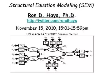
COV(X1,Y1) = g11s2x1 COV(Y1,Y2) = g11b21sx1y1 + g11g21s2X1 Back to the path model
SEM models • All of the relationships in the model are translatable into equations • Analysis in SEM is preceded by specifying a model like in the previous slide • This model is used to create an estimated covariance matrix
SEM models • The goal is to specify a model with an estimated covariance matrix that is not significantly different from the sample covariance matrix • CFA differs from EFA in that the difference can be tested using a Chi-square test • If ML methods are used in EFA a chi-square test can be estimated as well
Model Specification • Bentler-Weeks model • Matrices • B – Beta matrix, matrix of regression coefficients of DVs predicting other DVs • g – Gamma matrix, matrix of regression coefficients of DVs predicted by IVs • F – phi matrix, matrix of covariances among the IVs • - eta matrix, vector of DVs • - xi matrix, vector of IVs • Bentler-Weeks regression model
Model Specification • Bentler-Weeks model • Only independent variables have covariances (phi matrix) • This includes everything with a single headed arrow pointing away from it (e.g. E’s, F’s, V’s, D’s, etc.) • The estimated parameters are in the B, g and F matrices
Model Specification • Bentler-Weeks model matrix form
Model Specification • Phi Matrix • It is here that other covariances can be specified
Model Estimation • Model estimation in SEM requires start values • There are methods for generating good start values • Good means less iterations needed to estimate the model • Just rely on EQS or other programs to generate them for you (they do a pretty good job)
Model Estimation • These start values are used in the first round of model estimation by inserting them into the Bentler-Weeks model matrices (indicated by a “hat”) in place of the *s • Using EQS we get start values for the example
Model Estimation • Selection Matrices (G) • These are used to pull apart variables to use them in matrix equations to estimate the covariances • So that Y = Gy * and Y is only measured dependent variables
Model Estimation • Gx = [1 0 0 0 0 0 0] so that: X = Gx * and X is (are) the measured variable(s) • Rewriting the matrix equation to solve for we get: =(I-)-1 • This expresses the DVs as linear combinations of the IVs
Model Estimation • The estimated population covariance matrix for the DVs is found by:
Model Estimation • Estimated covariance matrix between DVs and IVs
The covariance(s) between IVs is estimated by : Model Estimation
Model Estimation • Programs like EQS usually estimate all parameters simultaneously giving an estimated covariance matrix sigma-hat • S is the sample covariance matrix • The residual matrix is found by subtracting sigma-hat from S • This whole process is iterative so that after the first iteration the values of the hat matrices output are input as new starting values
Model Estimation • Iterations continue until the function (usually ML) is minimized, this is called convergence • After five iterations the residual matrix in the example is:
Model Estimation • When the model converges you get estimates of all of the parameters and a converged residual matrix
Model Evaluation • 2 is based in the function minimum (from ML estimation) when the model converges • The minimum value is multiplied by N – 1 • From EQS: (.08924)(99) = 8.835 • The DFs are calculated as the difference between the number of data points (p(p + 1)/2) and the number of parameters estimated • In the example 5(6)/2 = 15, and there are 11 estimates leaving 4 degrees of freedom
Model Estimation • 2(4) = 8.835, p = .065 • The goal in SEM is to get a non-significant chi-square because that means there is little difference between the hypothesized and sample covariance matrices • Even with non-significant model you need to test significance of predictors • Each parameter is divided by its SE to get a Z-score which can be evaluated • SE values are best left to EQS to estimate
Final example model with (unstandardized) and standardized values Final Model