Exploring Polynomial Functions: Smooth Graphs & Zeros
310 likes | 428 Views
Learn about polynomial functions with smooth, continuous graphs. Understand the behavior, end behavior, zeros, and turning points. Use examples and strategies for graphing effectively.

Exploring Polynomial Functions: Smooth Graphs & Zeros
E N D
Presentation Transcript
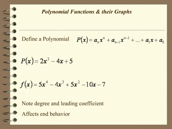
Polynomial functions of degree 2 or higher have graphs that are smooth and continuous. By smooth, we mean that the graphs contain only rounded curves with no sharp corners. By continuous, we mean that the graphs have no breaks and can be drawn without lifting your pencil from the rectangular coordinate system.
Odd-degree polynomial functions have graphs with opposite behavior at each end. Even-degree polynomial functions have graphs with the same behavior at each end.
Example Use the Leading Coefficient Test to determine the end behavior of the graph of f(x)= - 3x3- 4x + 7
Example Use the Leading Coefficient Test to determine the end behavior of the graph of f(x)= - .08x4- 9x3+7x2+4x + 7 This is the graph that you get with the standard viewing window. How do you know that you need to change the window to see the end behavior of the function? What viewing window will allow you to see the end behavior?
If f is a polynomial function, then the values of x for which f(x) is equal to 0 are called the zeros of f. These values of x are the roots, or solutions, of the polynomial equation f(x)=0. Each real root of the polynomial equation appears as an x-intercept of the graph of the polynomial function.
Example Find all zeros of x3+2x2- 4x-8=0
Graphing Calculator- Finding the Zeros x3+2x2- 4x-8=0 One zero of the function One of the zeros Other zero The other zero The x-intercepts are the zeros of the function. To find the zeros, press 2nd Trace then #2. The zero -2 has multiplicity of 2.
Example Find the zeros of f(x)=(x- 3)2(x-1)3 and give the multiplicity of each zero. State whether the graph crosses the x-axis or touches the x-axis and turns around at each zero. Continued on the next slide.
Example Now graph this function on your calculator. f(x)=(x- 3)2(x-1)3
Show that the function y=x3- x+5 has a zero between - 2 and -1.
Example Show that the polynomial function f(x)=x3- 2x+9 has a real zero between - 3 and - 2.
The graph of f(x)=x5- 6x3+8x+1 is shown below. The graph has four smooth turning points. The polynomial is of degree 5. Notice that the graph has four turning points. In general, if the function is a polynomial function of degree n, then the graph has at most n-1 turning points.
Example Graph f(x)=x4- 4x2 using what you have learned in this section.
Example Graph f(x)=x3- 9x2 using what you have learned in this section.
Use the Leading Coefficient Test to determine the end behavior of the graph of the polynomial function f(x)=x3- 9x2 +27 (a) (b) (c) (d)
State whether the graph crosses the x-axis, or touches the x-axis and turns around at the zeros of 1, and - 3. f(x)=(x-1)2(x+3)3 (a) (b) (c) (d)