Optimizing Cache Performance in Matrix Multiplication
Explore optimization techniques in matrix multiplication to improve high performance computing algorithms. Learn about cache performance, memory models, and machine efficiency considerations to enhance implementation quality.

Optimizing Cache Performance in Matrix Multiplication
E N D
Presentation Transcript
Optimizing Cache Performancein Matrix Multiplication UCSB CS240A, 2017 Modified from Demmel/Yelick’s slides
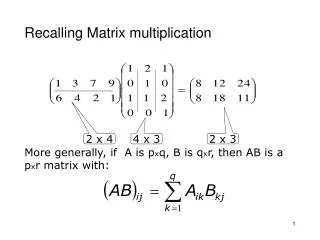
Case Study with Matrix Multiplication • An important kernel in many problems • Optimization ideas can be used in other problems • The most-studied algorithm in high performance computing • How to measure quality of implementation in terms of performance? • Megaflops number • Defined as: Core computation count / time spent • Matrix-matrix multiplication operation count = 2 n^3 • Example: 300MFLOPS 300 million MM-related floating operations performed per second.
What do commercial and CSE applications have in common? (Red Hot Blue Cool)
Matrix-multiply, optimized several ways Speed of n-by-n matrix multiply on Sun Ultra-1/170, peak = 330 MFlops
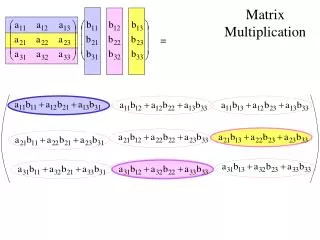
Note on Matrix Storage • A matrix is a 2-D array of elements, but memory addresses are “1-D” • Conventions for matrix layout • by column, or “column major” (Fortran default); A(i,j) at A+i+j*n • by row, or “row major” (C default) A(i,j) at A+i*n+j • recursive later) • Column major (for now) Column major matrix in memory Row major Column major 0 5 10 15 0 1 2 3 1 6 11 16 4 5 6 7 2 7 12 17 8 9 10 11 3 8 13 18 12 13 14 15 4 9 14 19 16 17 18 19 Blue row of matrix is stored in red cachelines cachelines Figure source: Larry Carter, UCSD
Computational Intensity: Key to algorithm efficiency Machine Balance: Key to machine efficiency Using a Simple Model of Memory to Optimize • Assume just 2 levels in the hierarchy, fast and slow • All data initially in slow memory • m = number of memory elements (words) moved between fast and slow memory • tm = time per slow memory operation • f = number of arithmetic operations • tf = time per arithmetic operation << tm • q = f / m average number of flops per slow memory access • Minimum possible time = f* tf when all data in fast memory • Actual time = computation cost + data fetch cost • f * tf + m * tm = f * tf * (1 + tm/tf * 1/q) • Larger q means time closer to minimum f * tf • q tm/tfneeded to get at least half of peak speed
Warm up: Matrix-vector multiplication {implements y = y + A*x} for i = 1 to n for j = 1 to n y(i) = y(i) + A(i,j)*x(j) A(i,:) + = * y(i) y(i) x(:)
Warm up: Matrix-vector multiplication {read x(1:n) into fast memory} {read y(1:n) into fast memory} for i = 1 to n {read row i of A into fast memory} for j = 1 to n y(i) = y(i) + A(i,j)*x(j) {write y(1:n) back to slow memory} • m = number of slow memory refs = 3n + n2 • f = number of arithmetic operations = 2n2 • q = f / m2 • Time • f * tf + m * tm = f * tf * (1 + tm/tf * 1/q) • = 2*n2 * tf * (1 + tm/tf * 1/2) • Megaflop rate =f/ Time = 1 / (tf + 0.5 tm) • Matrix-vector multiplication limited by slow memory speed
Modeling Matrix-Vector Multiplication • Compute time for nxn = 1000x1000 matrix • For tf and tm, using data from R. Vuduc’s PhD (pp 351-3) • http://bebop.cs.berkeley.edu/pubs/vuduc2003-dissertation.pdf • For tm use minimum-memory-latency / words-per-cache-line machine balance (q must be at least this for ½ peak speed)
Simplifying Assumptions • What simplifying assumptions did we make in this analysis? • Ignored parallelism in processor between memory and arithmetic within the processor • Sometimes drop arithmetic term in this type of analysis • Assumed fast memory was large enough to hold three vectors • Reasonable if we are talking about any level of cache • Not if we are talking about registers (~32 words) • Assumed the cost of a fast memory access is 0 • Reasonable if we are talking about registers • Not necessarily if we are talking about cache (1-2 cycles for L1) • Memory latency is constant • Could simplify even further by ignoring memory operations in X and Y vectors • Megaflop rate = 1 / ( tf + 0.5 tm)
Validating the Model • How well does the model predict actual performance? • Actual DGEMV: Most highly optimized code for the platform • Model sufficient to compare across machines • But under-predicting on most recent ones due to latency estimate
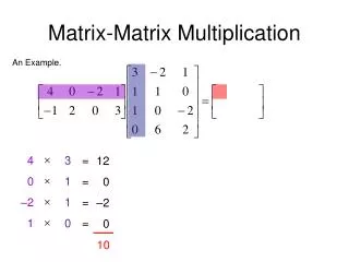
Naïve Matrix-Matrix Multiplication {implements C = C + A*B} for i = 1 to n for j = 1 to n for k = 1 to n C(i,j) = C(i,j) + A(i,k) * B(k,j) Algorithm has 2*n3 = O(n3) Flops and operates on 3*n2 words of memory q potentially as large as 2*n3 / 3*n2 = O(n) A(i,:) C(i,j) C(i,j) B(:,j) = + *
Naïve Matrix Multiply {implements C = C + A*B} for i = 1 to n {read row i of A into fast memory} for j = 1 to n {read C(i,j) into fast memory} {read column j of B into fast memory} for k = 1 to n C(i,j) = C(i,j) + A(i,k) * B(k,j) {write C(i,j) back to slow memory} A(i,:) C(i,j) C(i,j) B(:,j) = + *
Naïve Matrix Multiply Number of slow memory references on unblocked matrix multiply m = n3 to read each column of B n times + n2 to read each row of A once + 2n2 to read and write each element of C once = n3 + 3n2 So q = f / m = 2n3 / (n3 + 3n2) 2 for large n, no improvement over matrix-vector multiply Inner two loops are just matrix-vector multiply, of row i of A times B Similar for any other order of 3 loops A(i,:) C(i,j) C(i,j) B(:,j) = + *
Partitioning for blocked matrix multiplication • Example of submartix partitioning
Blocked (Tiled) Matrix Multiply Consider A,B,C to be N-by-N matrices of b-by-b subblocks where b=n / N is called the block size for i = 1 to N for j = 1 to N for k = 1 to N C(i,j) = C(i,j) + A(i,k) * B(k,j) {do a matrix multiply on blocks} A(i,k) C(i,j) C(i,j) = + * B(k,j)
Blocked (Tiled) Matrix Multiply Consider A,B,C to be N-by-N matrices of b-by-b subblocks where b=n / N is called the block size for i = 1 to N for j = 1 to N {read block C(i,j) into fast memory} for k = 1 to N {read block A(i,k) into fast memory} {read block B(k,j) into fast memory} C(i,j) = C(i,j) + A(i,k) * B(k,j) {do a matrix multiply on blocks} {write block C(i,j) back to slow memory} A(i,k) C(i,j) C(i,j) = + * B(k,j)
Blocked (Tiled) Matrix Multiply Recall: m is amount memory traffic between slow and fast memory matrix has nxn elements, and NxN blocks each of size bxb f is number of floating point operations, 2n3 for this problem q = f / m is our measure of memory access efficiency So: m = N*n2 read each block of B N3 times (N3 * b2 = N3 * (n/N)2 = N*n2) + N*n2 read each block of A N3 times + 2n2 read and write each block of C once = (2N + 2) * n2 So computational intensity q = f / m = 2n3 / ((2N + 2) * n2) n / N = b for large n So we can improve performance by increasing the blocksize b Can be much faster than matrix-vector multiply (q=2)
Using Analysis to Understand Machines The blocked algorithm has computational intensity q b • The larger the block size, the more efficient our algorithm will be • Limit: All three blocks from A,B,C must fit in fast memory (cache), so we cannot make these blocks arbitrarily large • Assume your fast memory has size Mfast 3b2 Mfast, so q b (Mfast/3)1/2 • To build a machine to run matrix multiply at 1/2 peak arithmetic speed of the machine, we need a fast memory of size Mfast 3b2 3q2 = 3(tm/tf)2 • This size is reasonable for L1 cache, but not for register sets • Note: analysis assumes it is possible to schedule the instructions perfectly
Basic Linear Algebra Subroutines (BLAS) • Industry standard interface (evolving) • www.netlib.org/blas, www.netlib.org/blas/blast--forum • Vendors, others supply optimized implementations • History • BLAS1 (1970s): • vector operations: dot product, saxpy (y=a*x+y), etc • m=2*n, f=2*n, q ~1 or less • BLAS2 (mid 1980s) • matrix-vector operations. Example: matrix vector multiply, etc • m=n^2, f=2*n^2, q~2, less overhead • somewhat faster than BLAS1 • BLAS3 (late 1980s) • matrix-matrix operations: Example: matrix matrix multiply, etc • m <= 3n^2, f=O(n^3), so q=f/m can possibly be as large as n, so BLAS3 is potentially much faster than BLAS2 • Good algorithms used BLAS3 when possible (LAPACK & ScaLAPACK) • Seewww.netlib.org/{lapack,scalapack} • If BLAS3 is not possible, use BLAS2 if applicable. Otherwise BLAS1.
BLAS speeds on an IBM RS6000/590 Peak speed = 266 Mflops Peak BLAS 3 BLAS 2 BLAS 1 BLAS 3 (n-by-n matrix matrix multiply) vs BLAS 2 (n-by-n matrix vector multiply) vs BLAS 1 (saxpy of n vectors)
Dense Linear Algebra: BLAS2 vs. BLAS3 • BLAS2 and BLAS3 have very different computational intensity, and therefore different performance Data source: Jack Dongarra
Summary • Performance programming on uniprocessors requires • understanding of memory system • understanding of fine-grained parallelism in processor • Simple performance models can aid in understanding • Two ratios are key to efficiency (relative to peak) • computational intensity of the algorithm: • q = f/m = # floating point operations / # slow memory references • machine balance in the memory system: • tm/tf = time for slow memory reference / time for floating point operation • Want q > tm/tf to get half machine peak • Blocking (tiling) is a basic approach to increase q • Techniques apply generally, but the details (e.g., block size) are architecture dependent • Similar techniques are possible on other data structures and algorithms
Questions You Should Be Able to Answer • What is the key to understand algorithm efficiency in our simple memory model? • Why does block matrix multiply reduce the number of memory references? 2D blocking is sometime called tiling • What are the BLAS?
Summary • Details of machine are important for performance • Processor and memory system (not just parallelism) • Before you parallelize, make sure you’re getting good serial performance • What to expect? Use understanding of hardware limits • Locality is at least as important as computation • Temporal: re-use of data recently used • Spatial: using data nearby that recently used • Machines have memory hierarchies • 100s of cycles to read from DRAM (main memory) • Caches are fast (small) memory that optimize average case • Can rearrange code/data to improve locality • Useful techniques: Blocking. Loop exchange.