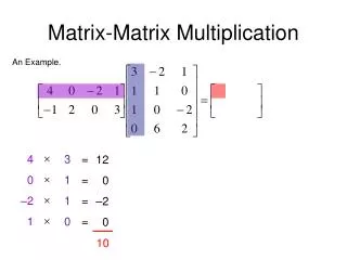
Matrix Multiplication
Matrix Multiplication. Instructor: Dr Sushil K Prasad Presented By: R. Jayampathi Sampath. Outline. Introduction Hypercube Interconnection Network The Parallel Algorithm Matrix Transposition Communication Efficient Matrix Multiplication on Hypercubes (The paper). Introduction.

Matrix Multiplication
E N D
Presentation Transcript
Matrix Multiplication Instructor: Dr Sushil K Prasad Presented By: R. Jayampathi Sampath
Outline • Introduction • Hypercube Interconnection Network • The Parallel Algorithm • Matrix Transposition • Communication Efficient Matrix Multiplication on Hypercubes (The paper)
Introduction • Matrix multiplication is important algorithm design in parallel computation. • Matrix multiplication on hypercube • Diameter is smaller • Degree = log(p) • Straightforward RAM algorithm for MatMul requires O(n3) time. • Sequential Algorithm: for (i=0; i<n; i++){ for (j=0; j<n; j++) { t=0; for(k = 0; k<n; k++){ t=t +aik*bkj; } cij=t; } }
Hypercube Interconnection Network 1101 1111 1100 0101 0100 0111 0110 0010 0000 0011 0001 1000 1011 1001
Hypercube Interconnection Network (contd.) • The formal specification of a Hypercube Interconnection Network. • Let processors be available • Let i and i(b) be two integers whose binary representation differ only in position b, • Specifically, • If is binary representation of i • Then is the binary representation of i(b) where is the complement of bit • A g-Dimentional Hypercube interconnection network is formed by connection each processor pi to by two way link for all
101 100 1 -1 2 -2 000 001 1 -1 2 -2 1 -1 2 -2 • 1 2 • 3 4 A = 2 -4 2 -3 010 011 2 -1 3 -3 4 -4 2 -2 3 -3 4 -4 • -1 -2 • -3 -4 B = 110 111 1 -1 1 -2 1 -1 1 -2 3 -3 4 -4 3 -1 3 -2 3 -3 3 -4 4 -3 4 -4 4 -3 4 -4 The Parallel Algorithm Initial step Step 1.1 Step1: • Example (parallel algorithm) A(0,j,k) & B(0,j,k) -> processors (i,j,k), where 1<=i<=n-1. 2*2 Step 1.2 n=21 #processors N N=n3=23=8 Step 1.2 A(i,j,i) -> processors (i,j,k) where 0<=k<=n-1 B(i,j,k) -> processors (i,j,k) where 0<=j<=n-1 X,X,X i j k
-8 -6 -1 -7 -2 -10 -3 -15 -6 -22 -16 -12 The Parallel Algorithm (contd.) Step2: Step3:
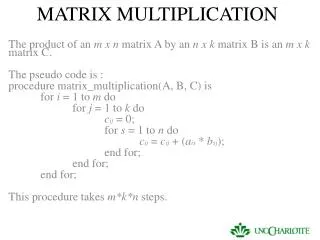
The Parallel Algorithm (contd.) • Implementation of straightforward RAM algorithm on HC. • The multiplication of two n x n matrices A , B where n=2q • Use HC with N = n3 = 23q • Each processor Pr occupying position (i,j,k) where r = in2 + jn + k for 0<= i,j,k <= n-1 • If the binary representation of r is : r3q-1r3q-2…r2qr2q-1…rqrq-1…r0 then the binary representation of i, j, k are r3q-1r3q-2…r2q,r2q-1…rq,rq-1…r0 respectively
The Parallel Algorithm (contd.) • Example (positioning) • The multiplication of two 2 x 2 matrices A , B where n=2=21 q=1 • Use HC with N = n3 = 23q=8 processors • Each processor Pr occupying position (i,j,k) • where r = i22 + j2 + k for 0<= i,j,k <= 1 • If the binary representation of r is : • r2r1r0 • then the binary representation of i, j, k are • r2,r1,r0 respectively
101 100 Ar 000 001 101 Br Cr 010 011 110 111 The Parallel Algorithm (contd.) • All processors with same index value in the one of i,j,k form a HC with n2 processors • All processors with the same index value in two field coordinates form a HC with n processors • Each processor will have 3 registers Ar, Br and Cralso denoted A(I,j,k) B(I,j,k) and C(i,j,k)
The Parallel Algorithm (contd.) • Step 1:The elements of A and B are distributed to the n3 processors so that the processor in position i,j,k will contain aji and bik • 1.1 Copies of data initially in A(0,j,k) and B(0,j,k) are sent to processors in positions (i,j,k), where 1<=i<=n-1. Resulting in A(i,j,k) = aij and B(i,j,k) = bjk for 0<=i<=n-1. • 1.2 Copies of data in A(i,j,i) are sent to processors in positions (i,j,k), where 0<=k<=n-1. Resulting in A(i,j,k) = aji for 0<=k<=n-1. • 1.3 Copies of data in B(i,j,k) are sent to processors in positions (i,j,k), where 0<=j<=n-1. Resulting in B(i,j,k) = bik for 0<=j<=n-1. • Step 2: Each processor in position (i,j,k) computes the product C(i,j,k) = A(i,j,k) * B(i,j,k) • Step 3: The sum C(0,j,k) = ∑C(i,j,k) for 0<=i<=n-1 and is computed for 0<=j,k<n-1.
The Parallel Algorithm (contd.) • Analysis • Steps 1.1,1.1,1.3 and 3 consists of q constant time iterations. • Step 2 requires constant time • So, T(n3) = O(q) = O(logn) • Cost pT(p) = O(n3logn) • Not cost optimal.
n=4=22 #processors N N=n3=43=64 XX,XX,XX i j k Copies of data initially in A(0,j,k) and B(0,j,k)
n=4=22 #processors N N=n3=43=64 XX,XX,XX i j k A(0,j,k) and B(0,j,k) are sent to processors in positions (i,j,k), where 1<=i<=n-1
n=4=22 #processors N N=n3=43=64 XX,XX,XX i j k Copies of data initially in A(0,j,k) and B(0,j,k)
n=4=22 #processors N N=n3=43=64 XX,XX,XX i j k Senders of A Copies of data in A(i,j,i) are sent to processors in positions (i,j,k), where 0<=k<=n-1
n=4=22 #processors N N=n3=43=64 XX,XX,XX i j k Senders of B Copies of data in B(i,j,k) are sent to processors in positions (i,j,k), where 0<=j<=n-1
Matrix Transposition • The number of processors used is N = n2 = 22q and processor Pr occupies position (i,j) where r = in + j where 0<=i,j<=n-1. • Initially, processor Pr holds all of the elements of matrix A where r = in + j. • Upon termination, processor Ps holds element aij where s = jn + i.
Matrix Transposition (contd.) • A recursive interpretation of the algorithm • Divide the matrix into 4 sub-matrices – n/2 x n/2 • The first level of recursion • The elements of bottom left sub-matrix are swapped with the corresponding elements of the top right sub-matrix. • The elements of other two sub-matrix are untouched. • The same step is now applied to each of four (n/2)*(n/2) matrices. • This continues until 2*2 matrices are transposed. • Analysis • The algorithm consists of q constant time iterations. • T(n) = log(n) • Cost = n2log(n) – not cost optimal (n(n-1)/2 operations on n*n matrix on the RAM by swapping aij wit aji for all i<j)
Matrix Transposition (contd.) • Example 1.1 1.0 1.3 1.2
Outline • 2D Diagonal Algorithm • The 3-D Diagonal Algorithm
2D Diagonal Algorithm A B 4*4 4*4 Step 1
2D Diagonal Algorithm (Contd.) Step 2 Step 3 Step 4
2D Diagonal Algorithm (Contd.) • Above algorithm can be extended to a 3-D mesh embedded in a hypercube with A*i and Bi* being initially distributed along the third dimension z. • Processor piik holding the sub-blocks of Akiand Bik • One-to-all-personalized broadcast of Bi* then replaced by point-to-point communication of Bik from piik to pkik • It fallows one-to-all broadcast Bik to pkik along the z direction.
The 3-D Diagonal Algorithm • HC consisting of p processors • Can be visualized as a 3-D mesh of size • Matrices A and B are partitioned into blocks of p⅔ with blocks along each dimension. • Initially, it is assumed that A and B are mapped onto the 2-D plane x = y • processor piik containing the blocks of Aki and Bki
The 3-D Diagonal Algorithm (contd.) • Algorithm consists of 3 phases • Point to point communication of Bki by piik to pikk • One to all broadcast of blocks of A along the x direction and the newly acquired block of B along the z direction. • Now processor pijk has the blocks of Akj and Bji • Each processor calculates the products of blocks of A and B. • The reduction by adding the result sub matrices along the z direction.
The 3-D Diagonal Algorithm (contd.) • Analysis • Phase 1: Passing messages of size n2/ p⅔ require log(3√p(ts + tw(n2/ p⅔ ))) where ts is the time it takes to start up for message sending and tw is time it takes to send a word from one processor to its neighbor. • Phase 2: takes twice as much time as phase 1. • Phase 3: Can be completed in the same amount of time as Phase 1. • Overall, the algorithm takes (4/3 log p, n2/ p⅔ (4/3 log p))
Bibliography • Akl, Parallel Computation, Models and Methods, Prentice Hall 1997. • Gupta, H & Sadayappan P., Communication Efficient Matrix Mulitplication on Hypercubes, August 1994 Proceedings of the sixth annual ACM symposium on Parallel algorithms and architectures, 320 - 329 • Quinn, M.J., Parallel Computing – Theory and Practice, McGraw Hill, 1997