Statistical Data Analysis: Lecture 7

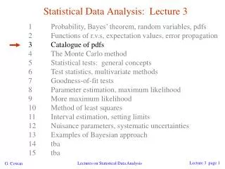
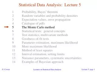
1. Statistical Data Analysis: Lecture 7 1 Probability, Bayes’ theorem, random variables, pdfs 2 Functions of r.v.s, expectation values, error propagation 3 Catalogue of pdfs 4 The Monte Carlo method 5 Statistical tests: general concepts 6 Test statistics, multivariate methods 7 Significance tests 8 Parameter estimation, maximum likelihood 9 More maximum likelihood 10 Method of least squares 11 Interval estimation, setting limits 12 Nuisance parameters, systematic uncertainties 13 Examples of Bayesian approach 14 tba Lectures on Statistical Data Analysis

2. Testing significance / goodness-of-fit for a set of Suppose hypothesis H predicts pdf observations We observe a single point in this space: What can we say about the validity of H in light of the data? Decide what part of the data space represents less compatibility with H than does the point more compatible with H less compatible with H (Not unique!) Lectures on Statistical Data Analysis

3. p-values Express ‘goodness-of-fit’ by giving the p-value for H: p = probability, under assumption of H, to observe data with equal or lesser compatibility with H relative to the data we got. This is not the probability that H is true! In frequentist statistics we don’t talk about P(H) (unless H represents a repeatable observation). In Bayesian statistics we do; use Bayes’ theorem to obtain where p (H) is the prior probability for H. For now stick with the frequentist approach; result is p-value, regrettably easy to misinterpret as P(H). Lectures on Statistical Data Analysis

4. p-value example: testing whether a coin is ‘fair’ Probability to observe n heads in N coin tosses is binomial: Hypothesis H: the coin is fair (p = 0.5). Suppose we toss the coin N = 20 times and get n = 17 heads. Region of data space with equal or lesser compatibility with H relative to n = 17 is: n = 17, 18, 19, 20, 0, 1, 2, 3. Adding up the probabilities for these values gives: i.e. p = 0.0026 is the probability of obtaining such a bizarre result (or more so) ‘by chance’, under the assumption of H. Lectures on Statistical Data Analysis

5. The significance of an observed signal Suppose we observe n events; these can consist of: nb events from known processes (background) ns events from a new process (signal) If ns, nb are Poisson r.v.s with means s, b, then n = ns + nb is also Poisson, mean = s + b: Suppose b = 0.5, and we observe nobs = 5. Should we claim evidence for a new discovery? Give p-value for hypothesis s = 0: Lectures on Statistical Data Analysis

6. Significance from p-value Often define significance Z as the number of standard deviations that a Gaussian variable would fluctuate in one direction to give the same p-value. 1 - TMath::Freq TMath::NormQuantile Lectures on Statistical Data Analysis

7. The significance of a peak Suppose we measure a value x for each event and find: Each bin (observed) is a Poisson r.v., means are given by dashed lines. In the two bins with the peak, 11 entries found with b = 3.2. The p-value for the s = 0 hypothesis is: Lectures on Statistical Data Analysis

8. The significance of a peak (2) But... did we know where to look for the peak? → give P(n ≥ 11) in any 2 adjacent bins Is the observed width consistent with the expected x resolution? → take x window several times the expected resolution How many bins  distributions have we looked at? →look at a thousand of them, you’ll find a 10-3 effect Did we adjust the cuts to ‘enhance’ the peak? →freeze cuts, repeat analysis with new data How about the bins to the sides of the peak... (too low!) Should we publish???? Lectures on Statistical Data Analysis

9. When to publish HEP folklore is to claim discovery when p = 2.9  10-7, corresponding to a significance Z = 5. This is very subjective and really should depend on the prior probability of the phenomenon in question, e.g., phenomenon reasonable p-value for discovery D0D0 mixing ~0.05 Higgs ~ 10-7 (?) Life on Mars ~10-10 Astrology ~10-20 One should also consider the degree to which the data are compatible with the new phenomenon, not only the level of disagreement with the null hypothesis; p-value is only first step! Lectures on Statistical Data Analysis

10. Distribution of the p-value The p-value is a function of the data, and is thus itself a random variable with a given distribution. Suppose the p-value of H is found from a test statistic t(x) as The pdf of pH under assumption of H is g(pH|H′) In general for continuous data, under assumption of H, pH ~ Uniform[0,1] and is concentrated toward zero for Some (broad) class of alternatives. g(pH|H) pH 0 1 Lectures on Statistical Data Analysis

11. Using a p-value to define test of H0 So the probability to find the p-value of H0, p0, less than a is We started by defining critical region in the original data space (x), then reformulated this in terms of a scalar test statistic t(x). We can take this one step further and define the critical region of a test of H0 with size a as the set of data space where p0≤ a. Formally the p-value relates only to H0, but the resulting test will have a given power with respect to a given alternative H1. Lectures on Statistical Data Analysis

12. Pearson’s c2 statistic Test statistic for comparing observed data (ni independent) to predicted mean values (Pearson’s c2 statistic) c2 = sum of squares of the deviations of the ith measurement from the ith prediction, using si as the ‘yardstick’ for the comparison. For ni~ Poisson(ni) we have V[ni] = ni, so this becomes Lectures on Statistical Data Analysis

13. Pearson’s c2 test If ni are Gaussian with mean niand std. dev. si, i.e., ni ~ N(ni, si2), then Pearson’s c2 will follow the c2 pdf (here for c2 = z): If the ni are Poisson with ni>> 1 (in practice OK for ni> 5) then the Poisson dist. becomes Gaussian and therefore Pearson’s c2 statistic here as well follows the c2 pdf. The c2 value obtained from the data then gives the p-value: Lectures on Statistical Data Analysis

14. The ‘c2 per degree of freedom’ Recall that for the chi-square pdf for N degrees of freedom, This makes sense: if the hypothesized ni are right, the rms deviation of ni from ni is si, so each term in the sum contributes ~ 1. One often sees c2/N reported as a measure of goodness-of-fit. But... better to give c2and N separately. Consider, e.g., i.e. for N large, even a c2 per dof only a bit greater than one can imply a small p-value, i.e., poor goodness-of-fit. Lectures on Statistical Data Analysis

15. Pearson’s c2 with multinomial data If is fixed, then we might model ni ~ binomial with pi = ni / ntot. I.e. ~ multinomial. In this case we can take Pearson’s c2 statistic to be If all pintot >> 1 then this will follow the chi-square pdf for N-1 degrees of freedom. Lectures on Statistical Data Analysis

16. Example of a c2 test ← This gives for N = 20 dof. Now need to find p-value, but... many bins have few (or no) entries, so here we do not expect c2 to follow the chi-square pdf. Lectures on Statistical Data Analysis

17. Using MC to find distribution of c2 statistic The Pearson c2 statistic still reflects the level of agreement between data and prediction, i.e., it is still a ‘valid’ test statistic. To find its sampling distribution, simulate the data with a Monte Carlo program: Here data sample simulated 106 times. The fraction of times we find c2 > 29.8 gives the p-value: p = 0.11 If we had used the chi-square pdf we would find p = 0.073. Lectures on Statistical Data Analysis

18. Wrapping up lecture 7 We’ve had a brief introduction to significance tests: p-value expresses level of agreement between data and hypothesis. p-value is not the probability of the hypothesis! p-value can be used to define a critical region, i.e., region of data space where p < α. We saw the widely used c2 test: statistic = sum of (data - prediction)2 / variance. Often c2~ chi-square pdf → use to get p-value. (Otherwise may need to use MC.) Next we’ll turn to the second main part of statistics: parameter estimation Lectures on Statistical Data Analysis